Uniform Cubic B-Spline Curves
Copyright © 2003-22, Howard J. Hamilton, University of Regina
Uniform Cubic B-Spline Curves: The General Idea - exam
There is some material in the textbook (Parent, R., Computer Animation: Algorithms and Techniques, Third Edition, Morgan Kaufmann, 2012) in Appendix B.5.12, but most of this material does not appear in the textbook.
If we assume that a series of segments from cubic functions will give a nice curve, then we can use the following general equation for the curve:
C(u) = a3u3 + a2u2 + a1u + a0
where a0, a1, a2, and a3 are parameters.
Let Q be the function composed of the segments. The value of u varies from 0 to 1 for each curve segment.
Q(u) = a3u3 + a2u2 + a1u + a0
for u = 0 to 1 for each segment.
Uniform cubic B-spline curves are based on the assumption that a nice curve corresponds to using cubic functions for each segment and constraining the points that joint the segments to meet three continuity requirements:
1. Positional Continuity (0 order): i.e. the end point of segment i is the same as the starting point of segment i + 1.
2. Tangential Continuity (1st order): i.e. no abrupt change in slope occurs at the transition between segment i and segment i + 1.
3. Curvature Continuity (2nd order): i.e. no polarity changes in slope at the transition between segment i and segment i + 1.
The curve Q is not constrained to pass through the given points. Therefore, the given points are referred to here as control points, i.e., they are points that control the shape of the curve, but they may not be on the curve themselves.
From the continuity requirements and the assumption that the weights total to 1 at all times, the following weighting functions (called basis functions) can be derived for 4 control points:
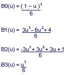
The B0, B1, B2, and B3 weighting functions tell us how much weight is assigned to points P0, P1, P2, and P3, respectively, depending on the value of u.
A way of deriving the above equations is shown later. For now, let’s consider what these functions are like.
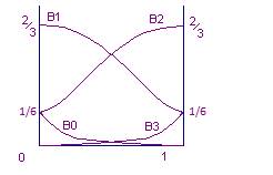
Here is an approximate graph (drawn by a person) of these functions on a single curve segment where u varies from 0 to 1:
Uniform B-Spline Approximation - exam
· not really “Interpolation”, since the curve does not pass through the points.
Suppose that we had 8 control points named P0 to P7. We can define 5 segments using groups of 4 consecutive points:
P0, P1, P2, P3;
P1, P2, P3, P4;
P2, P3, P4, P5;
P3, P4, P5, P6;
P4, P5, P6, P7
First, we want to find the curve segment, part of Q, defined by the points P0, P1, P2, and P3 (the real segment will be closer to P1 and P2 than the curve segment shown from Q0 to Q1 on the diagram):
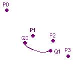
u = a parameter that ranges from 0 to 1 as we move along the curve segment. For example, if we do it in 100 steps, u goes from 0.00, 0.01, …, 1.00.
As we move from u = 0 to u = 1, the weights on the four points adjust smoothly. B0 goes from a weight of 1/6 gradually down to 0, B1 goes from 2/3 to 1/6, B2 goes from 1/6 to 2/3, and B3 goes from 0 to 1/6. From another point of view:
· B0 exchanges weights with B3 (1/6 is exchanged for 0)
· B1 exchanges weights with B2 (2/3 is exchanged for 1/6).
Recall that in graph form the functions look as follows on the interval:
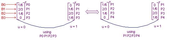
In vector form:
Example:
We see that when u = 0:
B0 (0) = (1 – u)3/6 = (1 – 0) 3/6 = 1/6
B1 (0) = (3u3 – 6u2 + 4)/6 = (0 – 0 + 4)/6 = 2/3
B2 (0) = ( –3u3 + 3u2 + 3u + 1)/6 = (0 + 0 + 0 + 1)/6 = 1/6
B3 (0) = u3/6 = 03/6 = 0
And when u = 1:
B0 (1) = (1 – u)3/6 = (1 – 1) 3/6 = 0
B1 (1) = (3u3 – 6u2 + 4)/6 = (3*1 – 6 + 4)/6 = 1/6
B2 (1) = ( –3u3 + 3u2 + 3u + 1)/6 = (–3 + 3 + 3 + 1)/6 = 2/3
B3 (1) = u3/6 = 13/6 = 1/6
We can also calculate any intermediate point, such as 0.5:
B0 (0.5) = (1 – 0.5) 3/6 = (1/2)3/6 = (1/8)/6 = 1/48
B1 (0.5) = (3/8 – 6/4 + 4)/6 = (3 – 12 + 32)/48 = 23/48
B2 (0.5) = (-3/8 + 3/4 + 3/2 + 1)/6 = (-3 + 6 +12 +8)/48 = 23/48
B3 (0.5) = (1/2)3/6 = (1/8)/6 = 1/48
The B weighting functions were designed so that the four parts must sum to 1 for every value of u from 0 to 1. For example: 1/6 + 2/3 + 1/6 + 0 = 1 and 1/48 + 23/48 + 23/48 + 1/48 = 1 in the above examples.
In the following equation:
the columns in the matrix (multiplied by 1/6) correspond to the equations:
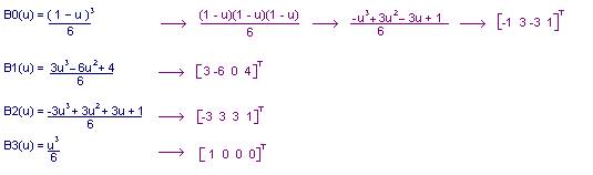
For example, the first column [-1, 3, -3, 1]T corresponds to B0.
The above equation guarantees Positional Continuity (0th order), Tangential Continuity (1st order), and Curvature Continuity (2nd order), as can be understood from how the equations were derived.
Deriving the Weighting Functions (B Functions) - exam
We want four equations, each a cubic with four unknowns. Thus, 16 unknowns must be found. One way is to find 16 equations and solve for the 16 unknowns.
Assumptions:
- The general form of the weight changes is known, but the specific constants (1/6 and 2/3) are not known.
o e.g., B0 goes from some value to nothing in interval
o e.g., B3 goes from nothing to the same value in interval
- B0 + B1 + B2 + B3 always sum to 1
- The B functions are the same in every interval
We will focus on one curve segment, where u varies from 0 to 1. From the positional continuity assumption, we get the following five equations:
B3 (0) = 0 (1)
B2 (0) = B3 (1) (2)
B1 (0) = B2 (1) (3)
B0 (0) = B1 (1) (4)
B0 (1) = 0 (5)
The meaning is that we want the value of B3 to be 0 at 0, the value of B2 at 0 to be the same as the value of B3 at 1, etc. Recall the diagram for the B functions, which is repeated below.
If we consider how one segment connects to the next, we can also state continuity requirements based on tangential and curvature continuity.
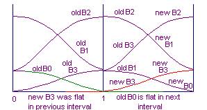
Here we’ve exaggerated the height of B0 and B3 in the middle of the curve segment to allow simpler visualization. First, note that after the end of the first interval, the B0 function for the first interval is flat (0). Thus, at u = 1, it is no longer changing. Its first and second derivatives should be zero.
B0’ (1) = 0 (6)
B0’’ (1) = 0 (7)
Similarly, before the beginning of the interval, B3 is flat. So at u = 0, it should be unchanging.
B3’ (0) = 0 (8)
B3’’ (0) = 0 (9)
We also want the first and second derivatives of B1 at u = 1 (Old B1 in the diagram) to match those of B0 at u = 0 (New B0). Since we want the basis functions to be the same in every interval, we get
B1’ (1) = B0’ (0) (10)
B1’’ (1) = B0’’ (0) (11)
We want the first and second derivatives of B2 at u = 1 (Old B2 in the diagram) to match those of B1 at u = 0 (New B1).
B2’ (1) = B1’ (0) (12)
B2’’ (1) = B1’’ (0) (13)
Similarly, for Old B3 and New B2
B3’ (1) = B2’ (0) (14)
B3’’ (1) = B2’’ (0) (15)
We now have a total of 15 equations. To get a 16th, an additional requirement was added: the sum of the B values should at all times be 1. It is sufficient to add the equation:
B0 (0) + B1 (0) + B2 (0) + B3 (0) = 1 (16)
Solving these 16 simultaneous equations gives the weighting functions previously presented.
B-Spline Program - exam
Intuition: for 2D, treat x and y separately, and for 3D, treat z in a similar manner.
Given:
![]()
We are interested in four consecutive control points at any one time.
Split each control point into two values:
Px[i], Px[i+1], Px[i+2], Px[i+3]
and
Py[i], Py[i+1], Py[i+2], Py[i+3]
Summation:
3
Qx(u) = ∑ Bk(u) * Px[i + k]
k = 0
3
Qy(u) = ∑ Bk(u) * Py[i + k]
k = 0
These two equations can be regarded as one vector equation:
3
Q(u) = ∑ Bk(u) * P [i + k]
k = 0
Write functions named B0, B1, B2, and B3 with parameter u. Recall that
Therefore, for example, function B0 is as follows.
function B0(u)
return (1 – u)* (1 – u) * (1 – u) / 6
Given the use of such functions, the uniform B-spline algorithm is as follows.
int MAX_STEPS = 100;
for (int i = 0; i < m - 3; i++)
{
for (int j = 0; j < MAX_STEPS; j++)
{
double u = j/MAX_STEPS;
Qx = B0 (u) * x[i] +
B1 (u) * x[i+1] +
B2 (u) * x[i+2] +
B3 (u) * x[i+3];
Qy = same as above only with y instead of x
// for 3d, Qz = same as above only with z instead of x
DrawPoint (Qx, Qy);
}
}
Why is the loop condition given as i < m – 3? Suppose m = 6, so the points are P0, P1, …, P5. We want to do P0, P1, P2, P3 and then P1, P2, P3, P4, and then P2, P3, P4, P5, so i is 0 then 1 and then 2. Thus, we want i < 3 when m = 6. In general, we want i < m - 3.
The above algorithm does not draw the very last point. We could fix this in several ways:
(1) Replace j < MAX_STEPS by j <= MAX_STEPS. This would draw the points where the curve segments join twice, but it would also draw the last point.
(2) Replace the second for statement with the following:
if (i == m – 4)
extra = 1;
else
extra = 0;
for (int j = 0; j < MAX_STEPS + extra; j++)
(3) Add extra draw statements after the end of the outer for loop to draw the last point
Qx = B0 (u) * x[m-4] +
B1 (u) * x[m-3] +
B2 (u) * x[m-2] +
B3 (u) * x[m-1];
Qy = …
DrawPoint(Qx, Qy)
Probably the simplest code to maintain is the first of these alternatives.
When u = 0, the plotted point will be quite close to P1, because P1 has 2/3 of the weight, while P0 and P2 each have only 1/6 of the weight and often, to some extent, cancel each other out. In the following diagram, the weights on each point are indicated along the x and y axes
NURBS = Non-Uniform Rational B-Splines – not on exam
- are a generalization of uniform B-Splines
- non-uniform means that instead of steadily advancing to the next four control points for each curve segment, sometimes we drop/add more data points. For uniform B-splines, the so-called knot vector, which tells us that the data points should be activated one per curve segment is [0, 1, 2, 3, 4, 5, 6, 7, 8, …], but for a non-uniform B-spline, it might be [0, 1, 2, 3, 4, 5, 5, 6, 7, …], which says that when the sixth control point is activated (corresponding to the first 5 in the knot vector), the seventh data point (corresponding to the second 5 in the knot vector) should also be activated.
- rational means that instead of every control point being weighted equally, control points have associated weights.