


Reference:
- 13. Findlater, L., and Hamilton, H.J. ``Iceberg Cube Algorithms: An Empirical Evaluation on Synthetic and Real Data,'' Intelligent Data Analysis, 7(2), 2003. Accepted April, 2002.
Introduction
An Iceberg-Cube contains only those cells of the data cube that meet an aggregate condition. It is called an Iceberg-Cube because it contains only some of the cells of the full cube, like the tip of an iceberg. The aggregate condition could be, for example, minimum support or a lower bound on average, min or max. The purpose of the Iceberg-Cube is to identify and compute only those values that will most likely be required for decision support queries. The aggregate condition specifies which cube values are more meaningful and should therefore be stored. This is one solution to the problem of computing versus storing data cubes.
For a three dimensional data cube, with attributes A, B and C, the Iceberg-Cube problem may be represented as:
FROM
CUBE BY
HAVING
TableName
A,B,C
COUNT(*)>=minsup
where minsup is the minimum support. Minimum support is the minimum number of tuples in which a combination of attribute values must appear to be considered frequent. It is expressed as a percentage of the total number of tuples in the input table.
When an Iceberg-Cube is constructed, it may also include those totals from the original cube that satisfy the minimum support requirement. The inclusion of totals makes Iceberg-Cubes more useful for extracting previously unknown relationships from a database.
For example, suppose minimum support is 25% and we want to create an Iceberg-Cube using Table 2 as input. For a combination of attribute values to appear in the Iceberg-Cube, it must be present in at least 25% of tuples in the input table, or 2 tuples. The resulting Iceberg-Cube is shown in Table 3. Those cells in the full cube whose counts are less than 2, such as ({P1, Vancouver, Vance},1), are not present in the Iceberg-Cube.
| Part | StoreLocation | Customer |
| P1 | Vancouver | Vance |
| P1 | Calgary | Bob |
| P1 | Toronto | Richard |
| P2 | Toronto | Allison |
| P2 | Toronto | Allison |
| P2 | Toronto | Tom |
| P2 | Ottawa | Allison |
| P3 | Montreal | Anne |
| Combination | Count |
| {P1, ANY, ANY} | 3 |
| {P2, ANY, ANY} | 4 |
| {ANY, Toronto, ANY} | 4 |
| {ANY, ANY, Allison} | 3 |
| {P2, Toronto, ANY} | 3 |
| {P2, ANY, Allison} | 3 |
| {ANY, Toronto, Allison} | 2 |
| {P2, Toronto, Allison} | 2 |
Methods for Computing Iceberg-Cubes
1. APRIORI
The APRIORI algorithm uses candidate combinations to avoid counting every possible combination of attribute values. For a combination of attribute values to satisfy the minimum support requirement, all subsets of that combination must also satisfy minimum support. The candidate combinations are found by combining only the frequent attribute value combinations that are already known. All other possible combinations are automatically eliminated because not all of their subsets would satisfy the minimum support requirement.
To do this, the algorithm first counts all single values on one pass of the data, then counts all candidate combinations of the frequent single values to identify frequent pairs. On the third pass over the data, it counts candidate combinations based on the frequent pairs to determine frequent 3-sets, and so on. This method guarantees that all frequent combinations of k values will be found in k passes over the database.
| A | B | C | D |
| a1 | b1 | c3 | d1 |
| a1 | b5 | c1 | d2 |
| a1 | b2 | c5 | d2 |
| a2 | b2 | c2 | d2 |
| a2 | b2 | c2 | d4 |
| a2 | b2 | c4 | d2 |
| a2 | b3 | c2 | d3 |
| a3 | b4 | c6 | d2 |
Table 4: Sample Input Table
| Combination | Count |
| {a1} | 3 |
| {a2} | 4 |
| {b2} | 4 |
| {c2} | 3 |
| {d2} | 5 |
| Combination |
| {a1,b2} |
| {a1,c2} |
| {a1,d2} |
| {a2, b2} |
| {a2,c2} |
| {a2,d2} |
| {b2,c2} |
| {b2,d2} |
| {c2,d2} |
| Combination | Count |
| {a1,d2} | 2 |
| {a2,b2} | 3 |
| {a2,c2} | 3 |
| {b2,c2} | 2 |
| {a2,d2} | 2 |
| {b2,d2} | 3 |
| Combination |
| {a2,b2,c2} |
| {a2,b2,d2} |
| Combination | Count |
| {a2,b2,c2} | 2 |
| {a2,b2,d2} | 2 |
2. Top-Down Computation
Top-down computation (tdC) computes an Iceberg-Cube by traversing down a multi-dimensional lattice formed from the attributes in an input table. The lattice represents all combinations of input attributes and the relationships between those combinations. Figure 10 shows a 4-Dimensional lattice of this type. The processing path of tdC is shown in Figure 11. The algorithm begins by computing the frequent attribute value combinations for the attribute set at the top of the tree, in this case ABCD. On the same pass over the data, tdC counts value combinations for ABCD, ABC, AB and A, adding the frequent ones to the Iceberg-Cube. This is facilitated by first ordering the database by the current attribute combination, ABCD. tdC then continues to the next leaf node in the tree, ABD, and counts those attribute value combinations. For n attributes, there are 2n-1 possible combinations of those attributes, which are represented as the leaf nodes in the tree. If no pruning occurs, then tdC examines every leaf node, making 2n-1 passes over the data. Pruning can occur when no attribute value combinations are found to be frequent for a certain combination of attributes. For example, if after the combination ABCD is processed, and there are no attribute value combinations of AB that are frequent, then tdC can prune the ABD node from the processing tree because all combinations that would be counted would start with AB, except for the single attribute A, which has already been counted.
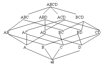
Figure 10: 4-Dimensional Lattice
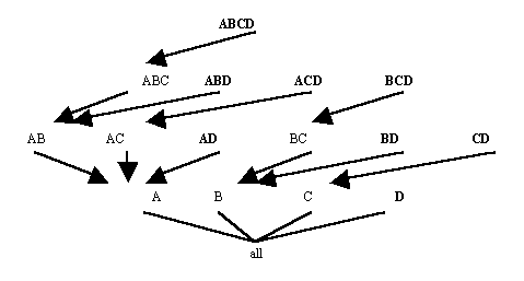
Figure 11: Processing Tree of tdC for Four Attributes
| A | B | C | D |
| a1 | b1 | c3 | d1 |
| a1 | b2 | c5 | d2 |
| a1 | b5 | c1 | d2 |
| a2 | b2 | c2 | d2 |
| a2 | b2 | c2 | d4 |
| a2 | b2 | c4 | d2 |
| a2 | b3 | c2 | d3 |
| a3 | b4 | c6 | d2 |
| Combination | Count |
| {a1} | 3 |
| {a2,b2,c2} | 2 |
| {a2,b2} | 3 |
| {a2} | 4 |
| A | B | D |
| a1 | b1 | d1 |
| a1 | b2 | d2 |
| a1 | b5 | d2 |
| a2 | b2 | d2 |
| a2 | b2 | d2 |
| a2 | b2 | d4 |
| a2 | b3 | d3 |
| a3 | b4 | d2 |
| Combination | Count |
| {a1} | 3 |
| {a2,b2,d2} | 2 |
| {a2,b2} | 3 |
| {a2} | 4 |
| Combination | Count |
| {a1} | 3 |
| {a2} | 4 |
| {a2,b2} | 3 |
| {a2,b2,c2} | 2 |
| {a2,b2,d2} | 2 |
| {a2,c2} | 3 |
| {a1,d2} | 2 |
| {a2,d2} | 2 |
| {b2,c2} | 2 |
| {b2} | 4 |
| {b2,d2} | 3 |
| {c2} | 3 |
| {d2} | 5 |
The cardinality of an attribute is the number of distinct values that attribute has. The tdC algorithm prunes most efficiently when the input attributes are ordered from highest to lowest cardinality because it is more likely to prune the first attribute in that case.
3. Bottom-Up Computation
The bottom-up computation algorithm(BUC) repeatedly sorts the database as necessary to allow convenient partitioning and counting of the combinations without large main memory requirements. BUC begins by counting the frequency of the first attribute in the input table. The algorithm then partitions the database based on the frequent values of the first attribute, so that only those tuples that contain a frequent value for the first attribute are further examined. BUC then counts combinations of values for the first two attributes and again partitions the databse so only those tuples that contain frequent combinations of the first two attributes are further examined, and so on.
For a database with four attributes, A, B, C and D, the processing tree of the BUC algorithm is shown in Figure 12. As with the tdC processing tree, this is based on the 4-dimensional lattice from Figure 10. The algorithm examines attribute A, then partitions the database by the frequent values of A, sorting each partition by the next attribute, B, for ease of counting AB combinations. Within each partition, BUC counts combinations of attributes A and B. Again, once the frequent combinations are found, the database is partitioned, this time on frequent combinations of AB, and is sorted by attribute C. When no frequent combinations are found, the algorithm traverses back down the tree and ascends to the next node. For example, if there are no frequent combinations of AC, then BUC will examine combinations of AD next. In this way, BUC prunes passes over the data. As with the tdC algorithm, BUC prunes most efficiently when the attributes are ordered from highest to lowest cardinality.

Figure 12: Processing Tree of BUC for Four Attributes
| A | B | C | D |
| a2 | b2 | c2 | d2 |
| a2 | b2 | c2 | d4 |
| a2 | b2 | c4 | d2 |
| a2 | b3 | c2 | d3 |
| A | B | C | D |
| a2 | b2 | c2 | d2 |
| a2 | b2 | c2 | d4 |
| a2 | b2 | c4 | d2 |
| A | B | C | D |
| a2 | b2 | c2 | d2 |
| a2 | b2 | c2 | d4 |
| A | B | D |
| a2 | b2 | d2 |
| a2 | b2 | d2 |
| a2 | b2 | d4 |
Table 18: Partition of {a2,b2} on D
4. Other Methods
For some databases the number of candidate combinations required to fit in main memory by the APRIORI algorithm becomes too large. Apart from tdC and BUC, other new methods have attempted to solve this problem. Three of these are FP-Growth, Top-k BUC and H-Mine.
FP-growth attempts to avoid candidate generation and minimize main memory use by compressing the database into a specialized data structure called an FP-tree. Unfortunately, the recursively generated conditional databases created by FP-growth may still exceed main memory size for large databases.
Top-k BUC is a specialized form of BUC, used for finding combinations with average values exceeding a specified minimum average. The average is calculated based on the sum of the values for a related measure attribute divided by the count of values. Top-k BUC also uses an H-tree (hyper-tree) for this problem.
Another recent algorithm is the H-Mine algorithm, based on partitioning the database. This algorithm requires less main memory than APRIORI and FP-Growth but more than BUC.