


 |
Clustering |   |
Cluster analysis is the process of grouping objects into subsets that have meaning in the context of a particular problem. The objects are thereby organized into an efficient representation that characterizes the population being sampled. Unlike classification, clustering does not rely on predefined classes. Clustering is referred to as an unsupervised learning method because no information is provided about the "right answer" for any of the objects. It can uncover previously undetected relationships in a complex data set. Many applications for cluster analysis exist. For example, in a business application, cluster analysis can be used to discover and characterize customer groups for marketing purposes.
Two types of clustering algorithms are nonhierarchical and hierarchical. In nonhierarchical
clustering, such as the k-means algorithm, the relationship between clusters is undetermined.
Hierarchical clustering repeatedly links pairs of clusters until every data object is included in the hierarchy. With both
of these approaches, an important issue is how to determine the similarity between two objects, so that
clusters can be formed from objects with a high similarity to each other. Commonly, distance functions,
such as the Manhattan and Euclidian distance functions, are used to determine similarity.
A distance function yields a higher value for pairs of objects that are less similar to one another. Sometimes a
similarity function is used instead, which yields higher values for pairs that are more similar.
Distance Functions
Given two p-dimensional data objects i = (xi1,xi2, ...,xip) and j = (xj1,xj2, ...,xjp), the following common distance functions can be defined:
Euclidian Distance Function:When using the Euclidian distance function to compare distances, it is not necessary to calculate the square root because distances are always positive numbers and as such, for two distances, d1 and d2, Öd1 > Öd2 Û d1 > d2. If some of an object's attributes are measured along different scales, so when using the Euclidian distance function, attributes with larger scales of measurement may overwhelm attributes measured on a smaller scale. To prevent this problem, the attribute values are often normalized to lie between 0 and 1.
Manhattan Distance Function:
Other distance functions may be more appropriate for some data.
k-means Algorithm
The k-means algorithm is one of a group of algorithms called partitioning methods. The problem of partitional clustering can be formally stated as follows: Given n objects in a d-dimensional metric space, determine a partition of the objects into k groups, or clusters, such that the objects in a cluster are more similar to each other than to objects in different clusters. Recall that a partition divides a set into disjoint parts that together include all members of the set. The value of k may or may not be specified and a clustering criterion, typically the squared-error criterion, must be adopted.
The solution to this problem is straightforward. Select a clustering criterion, then for each data object
select the cluster that optimizes the criterion. The k-means algorithm initializes k clusters
by arbitrarily selecting one object to represent each cluster. Each of the remaining objects are assigned to a cluster and
the clustering criterion is used to calculate the cluster mean. These means are used as the new cluster points
and each object is reassigned to the cluster that it is most similar to. This continues until there is no longer
a change when the clusters are recalculated. The algorithm is shown in Figure 1.
k-means Algorithm:
b) Compute new cluster centers as mean value of the objects in each cluster. Until no change in cluster center calculation |
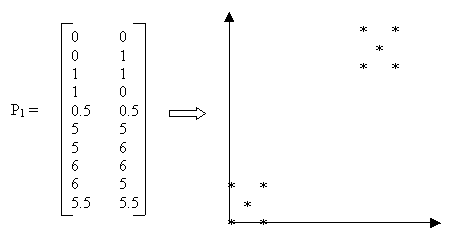
Example: Suppose we are given the data in Figure 2 as input and we choose k=2 and the Manhattan distance function dis = |x2-x1|+|y2-y1|. The detailed computation is as follows:
Step 1. Initialize k partitions. An initial partition can be formed by first specifying a set of k seed points. The seed points could be the first k objects or k objects chosen randomly from the input objects. We choose the first two objects as seed points and initialize the clusters as C1={(0,0)} and C2={(0,1)}.
Step 2. Since there is only one point in each cluster, that point is the cluster center.
Step 3a. Calculate the distance between each object and each cluster center, assigning the object to the closest cluster.
For example, for the third object:
dis(1,3) = |1-0| + |1-0| = 2 and
dis(2,3) = |1-0| + |1-1| = 1,
so this object is assigned to C2.
The fifth object is equidistant from both clusters, so we arbitrarily assign it to C1.
After calculating the distance for all points, the clusters contain the following objects:
C1 = {(0,0),(1,0),(0.5,0.5)} and
C2 = {(0,1),(1,1),(5,5),(5,6),(6,6),(6,5),(5.5,5.5)}.
Step 3b. Compute new cluster center for each cluster.
New center for C1 = (0.5,0.16)
(0+1+0.5)/3 = 0.5
(0+0+0.5)/3 = 0.16
New center for C2 = (4.1,4.2)
(0+1+5+5+6+6+5.5)/7 = 4.1
(1+1+5+5+6+6+5.5)/7 = 4.2
Step 3a'. New centers C1 = (0.5,0.16) and C2 = (4.1,4.2) differ from old centers C1={(0,0)} and C2={(0,1)}, so the loop is repeated.
Reassign the ten objects to the closest cluster center, resulting in:
C1 = {(0,0),(0,1),(1,1),(1,0),(0.5,0.5)}
C2 = {(5,5),(5,6),(6,6),(6,5),(5.5,5.5)}
Step 3b'. Compute new cluster center for each cluster
New center for C1 = (0.5,0.5)
New center for C2 = (5.5,5.5)
Step 3a''. New centers C1 = (0.5,0.5) and C2 = (5.5,5.5) differ from old centers C1 = (0.5,0.16) and C2 = (4.1,4.2), so the loop is repeated.
Reassign the ten objects to the closest cluster center. Result is same as in Step 5.
Step 3b''. Compute new cluster centers.
Algorithm is done: Centers are the same as in Step 3b', so algorithm is finished. Result is same as in 3b'.
Hierarchical algorithms can be either agglomerative or divisive, that is top-down or bottom-up. All agglomerative hierarchical clustering algorithms begin with each object as a separate group. These groups are successively combined based on similarity until there is only one group remaining or a specified termination condition is satisfied. For n objects, n-1 mergings are done. Hierarchical algorithms are rigid in that once a merge has been done, it cannot be undone. Although there are smaller computational costs with this, it can also cause problems if an erroneous merge is done. As such, merge points need to be chosen carefully. Here we describe a simple agglomerative clustering algorithm. More complex algorithms have been developed, such as BIRCH and CURE, in an attempt to improve the clustering quality of hierarchical algorithms.
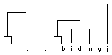
In the context of hierarchical clustering, the hierarchy graph is called a dendogram.
Figure 3 shows a sample dendogram that could be produced from a hierarchical clustering
algorithm. Unlike with the k-means algorithm, the number of clusters (k) is not specified
in hierarchical clustering. After the hierarchy is built, the user can specify the number of clusters
required, from 1 to n. The top level of the hierarchy represents one cluster, or k=1.
To examine more clusters, we simply need to traverse down the hierarchy.
|
Agglomerative Hierarchical Algorithm:
Given: A set X of objects {x1,...,xn} A distance function dis(c1,c2)
|
Figure 4 shows a simple hierarchical algorithm. The distance function in this algorithm can determine similarity of clusters through many methods, including single link and group-average. Single link calculates the distance between two clusters as the shortest distance between any two objects contained in those clusters. Group-average first finds the average values for all objects in the group (i.e., cluster) and the calculates the distance between clusters as the distance between the average values.
Each object in X is initially used to create a cluster containing a single object. These clusters are successively merged into new clusters, which are added to the set of clusters, C. When a pair of clusters is merged, the original clusters are removed from C. Thus, the number of clusters in C decreases until there is only one cluster remaining, containing all the objects from X. The hierarchy of clusters is implicity represented in the nested sets of C.
Example: Suppose the input to the simple agglomerative algorithm described above is the set X, shown in Figure 5 represented in matrix and graph form. We will use the Manhattan distance function and the single link method for calculating distance between clusters. The set X contains n=10 elements, x1 to x10, where x1=(0,0).* Agglomerative Hierarchical Algorithm adapted from: http://www.cs.columbia.edu/~regina/cs4999/notes/lec04/lec04-index.html.
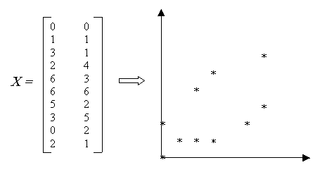
Figure 5: Sample Data
Step 1. Initially, each element xi of X is placed in a cluster ci, where ci is a member of the set of clusters C.
C = {{x1},{x2},{x3}, {x4},{x5},{x6},{x7}, {x8},{x9},{x10}}
Step 2. Set l = 11.
Step 3. (First iteration of while loop) C.size = 10Step 3. (Second iteration) C.size = 9
- The minimum single link distance between two clusters is 1. This occurs in two places, between c2 and c10 and between c3 and c10.
Depending on how our minimum function works we can choose either pair of clusters. Arbitrarily we choose the first.
(cmin1,cmin2) = (c2,c10)- Since l = 10, c11 = c2 U c10 = {{x2},{x10}}
- Remove c2 and c10 from C.
- Add c11 to C.
C = {{x1},{x3}, {x4},{x5},{x6},{x7}, {x8},{x9},{{x2}, {x10}}}- Set l = l + 1 = 12
Step 3. (Third iteration) C.size = 8
- The minimum single link distance between two clusters is 1. This occurs between, between c3 and c11 because the distance between x3 and x10 is 1, where x10 is in c11.
(cmin1,cmin2) = (c3,c11)- c12 = c3 U c11 = {{{x2},{x10}},{x3}}
- Remove c3 and c11 from C.
- Add c12 to C.
C = {{x1}, {x4},{x5},{x6},{x7}, {x8},{x9},{{{x2}, {x10}}, {x3}}}- Set l = 13
Step 3. (Fourth iteration) C.size = 7
- (cmin1,cmin2) = (c1,c12)
- C = {{x4},{x5},{x6},{x7}, {x8},{x9},{{{{x2}, {x10}}, {x3}},{x1}}}
Step 3. (Fifth iteration) C.size = 6
- (cmin1,cmin2) = (c4,c8)
- C = {{x5},{x6},{x7}, {x9},{{{{x2}, {x10}}, {x3}},{x1}},{{x4},{x8}}}
Step 3. (Sixth iteration) C.size = 5
- (cmin1,cmin2) = (c5,c7)
- C = {{x6}, {x9},{{{{x2}, {x10}}, {x3}},{x1}},{{x4},{x8}}, {{x5},{x7}}}
Step 3. (Seventh iteration) C.size = 4
- (cmin1,cmin2) = (c9,c13)
- C = {{x6}, {{x4},{x8}}, {{x5},{x7}},{{{{{x2}, {x10}}, {x3}},{x1}},{x9}}}
Step 3. (Eighth iteration) C.size = 3
- (cmin1,cmin2) = (c6,c15)
- C = {{{x4},{x8}}, {{{{{x2}, {x10}}, {x3}},{x1}},{x9}},{{x6}, {{x5},{x7}}}}
Step 3. (Ninth iteration) C.size = 2
- (cmin1,cmin2) = (c14,c16)
- C = { {{x6}, {{x5},{x7}}}, {{{x4},{x8}}, {{{{{x2}, {x10}}, {x3}},{x1}},{x9}}}}
Step 3. (Tenth iteration) C.size = 1. Algorithm done.
- (cmin1,cmin2) = (c17,c18)
- C = {{{{x4},{x8}}, {{{{{x2}, {x10}}, {x3}},{x1}},{x9}}}, {{x6}, {{x5},{x7}}}}
The cluster created from this algorithm can be seen in Figure 6. The corresponding dendogram formed from the hierarchy in C is shown in Figure 7. The points which appeared most closely together on the graph of input data in Figure 5 are grouped together more closely in the hierarchy.
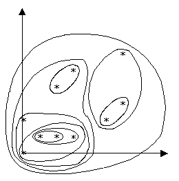
Figure 6: Graph with Clusters
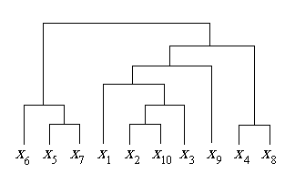
Figure 7: Sample Dendogram

|


|