


 |
Data Cubes |   |
Users of decision support systems often see data in the form of data
cubes. The cube is used to represent data along some measure of
interest. Although called a "cube", it can be 2-dimensional, 3-dimensional, or higher-dimensional. Each
dimension represents some attribute in the database and the cells in the data
cube represent the measure of interest. For example, they could contain a count
for the number of times that attribute combination occurs in the database, or
the minimum, maximum, sum or average value of some attribute. Queries are performed on the
cube to retrieve decision support information.
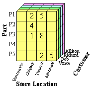
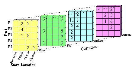
Example: We have a database that contains transaction information relating company sales of a part to a customer at a store location. The data cube formed from this database is a 3-dimensional representation, with each cell (p,c,s) of the cube representing a combination of values from part, customer and store-location. A sample data cube for this combination is shown in Figure 1. The contents of each cell is the count of the number of times that specific combination of values occurs together in the database. Cells that appear blank in fact have a value of zero. The cube can then be used to retrieve information within the database about, for example, which store should be given a certain part to sell in order to make the greatest sales.
|
|
Sample Data Cube |
Figure 1(b): Entire
View of |
The goal is to retrieve the
decision support information from the data cube in the most efficient way
possible. Three possible solutions are:
If the whole cube is pre-computed, then queries run on the cube will be very fast. The disadvantage is that the pre-computed cube requires a lot of memory. The size of a cube for n attributes A1,...,An with cardinalities |A1|,...,|An| is π|Ai|. This size increases exponentially with the number of attributes and linearly with the cardinalities of those attributes.
To minimize memory requirements, we can pre-compute none of the cells in the cube. The disadvantage here is that queries on the cube will run more slowly because the cube will need to be rebuilt for each query.
As a compromise between these two,
we can pre-compute only those cells in the cube which will most likely be used
for decision support queries. The trade-off between memory space and computing time is called
the space-time trade-off, and it often exists in data mining and computer science in general.
Representation
m-Dimensional Array:
A data cube built from m
attributes can be stored as an m-dimensional array. Each element of the
array contains the measure value, such as count. The array itself can be
represented as a 1-dimensional array. For example, a 2-dimensional array of
size x x y can be stored as a 1-dimensional array of size x*y,
where element (i,j) in the 2-D array is stored in location (y*i+j)
in the 1-D array. The disadvantage of storing the cube directly as an array is
that most data cubes are sparse, so the array will contain many empty elements (zero values).
List of Ordered Sets:
To save storage space we can store
the cube as a sparse array or a list of ordered sets. If we store all
cells in the data cube from Figure 1, then the resulting datacube will contain (cardPart
*cardStoreLocation*cardCustomer)
combinations, which is 5 * 4 * 4 = 80 combinations.
If we eliminate cells in the cube that contain zero, such as {P1, Vancouver, Allison},
only 27 combinations remain, as seen in Table 1.
Table 1 shows an ordered set representation of the data
cube. Each attribute value combination is paired with its corresponding count.
This representation can be easily stored in a database table to facilitate
queries on the data cube.
|
|
Table 1: Ordered Set Representation of a Data Cube
Another aspect of data cube representation which
can be considered is the representation
of totals. A simple data cube does not contain
totals. The storage of totals increases the size
of the data cube but can also decrease the
time to make total-based queries. A simple way to represent
totals is to add an additional layer on n sides of the n-dimensional datacube. This can
be easily visualized with the 3-dimensional data cube
introduced in Figure 1. Figure 2 shows the original
cube with an additional layer on each of three sides
to store total values. The totals represent the sum of all
values in one horizontal row, vertical row (column) or
depth row of the data cube.
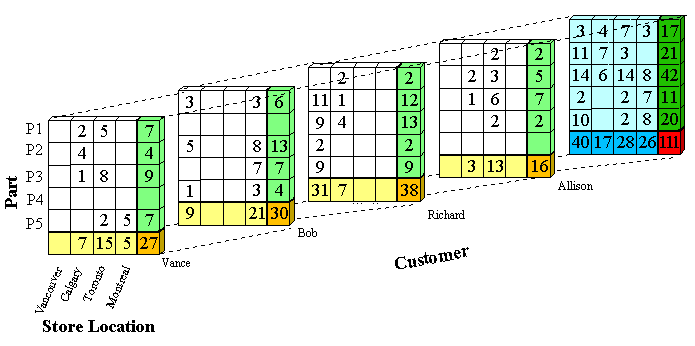
The color coding used in Figure 2 is as follows:
To store these totals in ordered set representation the value ANY can be used. For example,
there are 15 transactions where Vance buys a part in Toronto.
The ordered set representation of this
is ({ANY, Toronto, Vance},15),
because it could be any part.
The ordered set representation of all of Vance's
transactions is ({ANY, ANY, Vance},27), that is all transactions at all store locations for Vance.
The total number of transactions in the whole cube is found in the red cell and is 111. This is represented
as ({ANY, ANY, ANY}, 111).
Operations on Data Cubes
Summarization or Rollup
Rollup or summarization of the data cube can be done by traversing upwards through a concept hierarchy. A concept hierarchy maps a set of low level concepts to higher level, more general concepts. It can be used to summarize information in the data cube. As the values are combined, cardinalities shrink and the cube gets smaller. Generalizing can be thought of as computing some of the summary total cells that contain ANYs, and storing those in favour of the original cells.
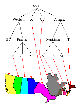
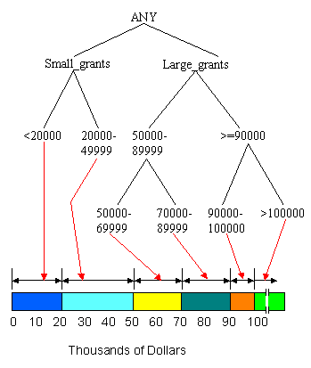
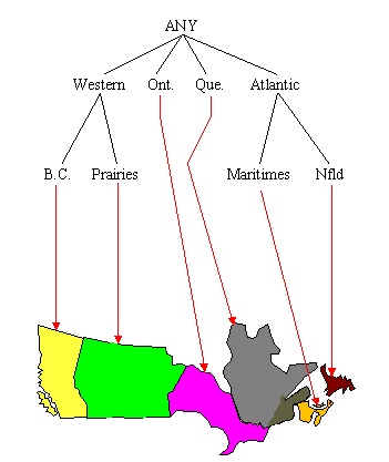
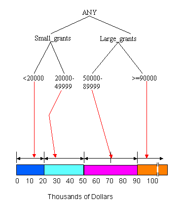
Figures 2 through 8 show an example of summarizing a data cube built from two attributes, Province and Grant_Amount. The measure of interest stored in the cube is Vote. It contains the total number of votes for each combination of Province and Grant_Amount that occurred in the input table. The concept hierarchies for the Province and Grant_Amount attributes are shown in Figure 2. In Figure 2(a), each province represents a location and some can be mapped to more general regions, such as the Prairies or the Maritimes. Those regions can be further mapped to Western Canada and Atlantic Canada. The top level of the hierarchy is "ANY", representing any location. Western and Atlantic Canada are higher level, more general concepts than, for example, Alberta and Nova Scotia. The concept hierarchy in Figure 2(b) represents the Grant_Amount dimension of the database. Grant_Amount is originally stored as specific numbers, such as $34000. The concept hierarchy generalizes the values by grouping them into categories of multiples of $10000, then $20000, and finally including all the amounts into ANY. Ordinarily, concept hierarchies are provided by a domain expert, because then the resulting general concepts will make sense to people familiar with the domain. Concept hierarchies might also be formed automatically by clustering.
|
|
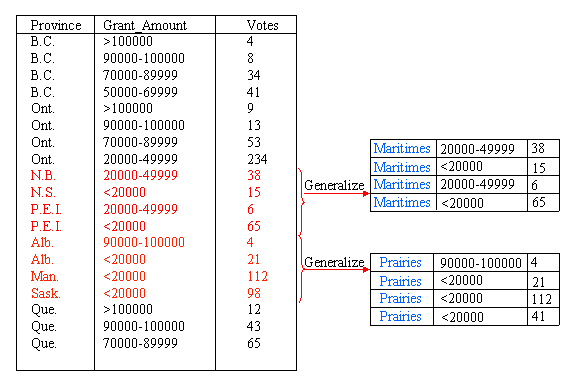
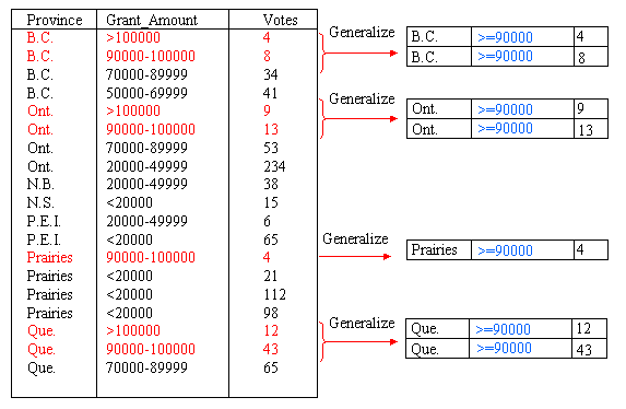
To reduce the size of the data cube, we can summarize the data by computing the cube at a higher level in the concept hierarchy. A non-summarized cube would be computed at the lowest level, for example, the province level in Figure 2(a). If we compute the cube at the second level, there are only six categories, B.C., Prairies, Ont., Que., Maritimes and Nfld., and the data cube will be much smaller. Figure 3 shows a sample generalization of the Province attribute for those provinces that can be grouped under the concept Prairies and those that can be grouped under the concept Maritimes. For example, for Sask., the province, or location name, changes to Prairies, but the other attribute values remain unchanged because they are not summarized at this point. The new, summarized concept hierarchy is shown in Figure 4.
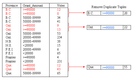
The next step in the process is to remove duplicate tuples from the data. The measure of interest, Votes, is summed for tuples that have the same Province and Grant_Amount values. For example, in Figure 5, three tuples contain the combination {Prairies, <20000}. The tuples are removed, their individual Votes values are summed, and a new tuple replaces all three, with a Votes value of 231.
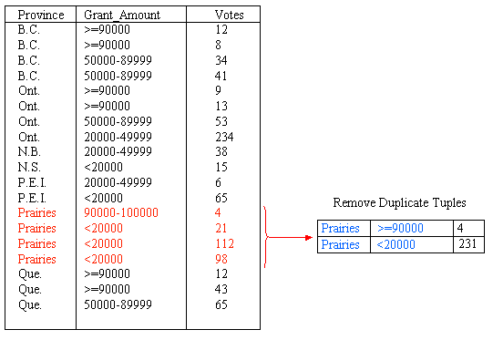
We can also generalize the Grant_Amount Attribute. Figure 6 shows summarization of this attribute through the addition of a new category for amounts greater than or equal to 90000. In total, the Grant_Amount value of seven tuples is changed to the new classification. After summarizing the data into groups of <20000, 20000 - 49999, 50000 - 89999 and >=90000, the concept hierarchy is as shown in Figure 7. Again, we need to remove the duplicate tuples after generalizating the Grant_Amount attribute. This is shown in Figure 8.
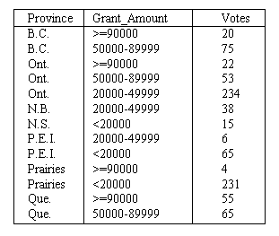
The final result of summarizing the data by introducing the categories Prairies, Maritimes and >=90000 is shown in Figure 9. From here, the process could be continued to further generalize Province or Grant_Amount.
Drill-down is similar
to Rollup, but is in reverse. A drill-down goes from less detailed data to more
detailed data. To drill-down, we can either traverse down a concept hierarchy
or add another dimension to the data cube. For example, given the data
shown in Figure 8, a drill-down on the Province attribute would result in more
detailed information about the location. The value Prairies would be replaced by the
more detailed values of Alberta, Saskatchewan and Manitoba. The result is the
data cube shown in Figure 7, before summarization. This is a reversal of the
summarization process.
Iceberg-Cubes
An Iceberg-Cube contains only those cells of the data cube that meet an aggregate condition. It is called an Iceberg-Cube because it contains only some of the cells of the full cube, like the tip of an iceberg. The aggregate condition could be, for example, minimum support or a lower bound on average, min or max. The purpose of the Iceberg-Cube is to identify and compute only those values that will most likely be required for decision support queries. The aggregate condition specifies which cube values are more meaningful and should therefore be stored. This is one solution to the problem of computing versus storing data cubes.
For a three dimensional data cube, with attributes A, B and C, the Iceberg-Cube problem may be represented as:
SELECT
FROM
CUBE BY
HAVINGA,B,C, Count(*),SUM(X)
TableName
A,B,C
COUNT(*)>=minsup,
where minsup is the minimum support. Minimum support is the minimum number of tuples in which a combination of attribute values must appear to be considered frequent. It is expressed as a percentage of the total number of tuples in the input table.
When an Iceberg-Cube is constructed, it may also include those totals from the original cube that satisfy the minimum support requirement. The inclusion of totals makes Iceberg-Cubes more useful for extracting previously unknown relationships from a database.
For example, suppose minimum support is 25% and we want to create an
Iceberg-Cube using Table 2 as input. For a combination of attribute values to
appear in the Iceberg-Cube, it must be present in at least 25% of tuples in the
input table, or 2 tuples. The resulting Iceberg-Cube is shown in Table 3. Those
cells in the full cube whose counts are less than 2, such as ({P1, Vancouver, Vance},1), are not present
in the Iceberg-Cube.
Table 2: Sample Database Table |
Table 3: Sample Iceberg-Cube with Minimum Support of at least 25% |
The APRIORI algorithm uses candidate combinations to avoid counting every possible combination of attribute values. For a combination of attribute values to satisfy the minimum support requirement, all subsets of that combination must also satisfy minimum support. The candidate combinations are found by combining only the frequent attribute value combinations that are already known. All other possible combinations are automatically eliminated because not all of their subsets would satisfy the minimum support requirement.
To do this, the algorithm first counts all single values on one pass of the data, then counts all candidate combinations of the frequent single values to identify frequent pairs. On the third pass over the data, it counts candidate combinations based on the frequent pairs to determine frequent 3-sets, and so on. This method guarantees that all frequent combinations of k values will be found in k passes over the database.
Example: Suppose the input table is as shown in Table 4. On the first pass over the data, the APRIORI algorithm determines that the single values shown in Table 5 are frequent. These single values are implicit representations of ordered sets in the ordered set representation of an Iceberg-Cube. For example, {a1} represents the combination {a1,ANY,ANY,ANY}. The candidate combinations that can be derived from these values are shown in Table 6. These combinations are counted on the second pass and the algorithm determines which of them are frequent. The result is shown in Table 7. From the frequent pairs, only one 3-set candidate combination can be derived, as shown in Table 8, and the algorithm counts this combination on the third pass over the data. The result of the third pass over the data is shown in Table 9. Since {a2, c2, d2} is not frequent no more candidate combinations can be derived, and the algorithm finishes execution.
| A | B | C | D |
| a1 | b1 | c3 | d1 |
| a1 | b5 | c1 | d2 |
| a1 | b2 | c5 | d2 |
| a2 | b2 | c2 | d2 |
| a2 | b2 | c2 | d4 |
| a2 | b2 | c4 | d2 |
| a2 | b3 | c2 | d3 |
| a3 | b4 | c6 | d2 |
Table 5: Combinations added after first pass. |
Table 6: Candidate combinations after first pass. |
Table 7: Combinations added after second pass. |
Table 8: Candidate combinations after second pass. |
Table 9: Combinations added after third pass. |
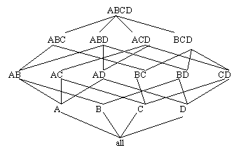
Top-down computation (TDC) computes an Iceberg-Cube by traversing down a multi-dimensional lattice formed from the attributes in an input table. The lattice represents all combinations of input attributes and the relationships between those combinations. Figure 10 shows a 4-Dimensional lattice of this type. The processing path of TDC is shown in Figure 11. The algorithm begins by computing the frequent attribute value combinations for the attribute set at the top of the tree, in this case ABCD. On the same pass over the data, TDC counts value combinations for ABCD, ABC, AB and A, adding the frequent ones to the Iceberg-Cube. This is facilitated by first ordering the database by the current attribute combination, ABCD. TDC then continues to the next leaf node in the tree, ABD, and counts those attribute value combinations. For n attributes, there are 2n-1 possible combinations of those attributes, which are represented as the leaf nodes in the tree. If no pruning occurs, then TDC examines every leaf node, making 2n-1 passes over the data. Pruning can occur when no attribute value combinations are found to be frequent for a certain combination of attributes. For example, if after the combination ABCD is processed, and there are no attribute value combinations of AB that are frequent, then TDC can prune the ABD node from the processing tree because all combinations that would be counted would start with AB, except for the single attribute A, which has already been counted.
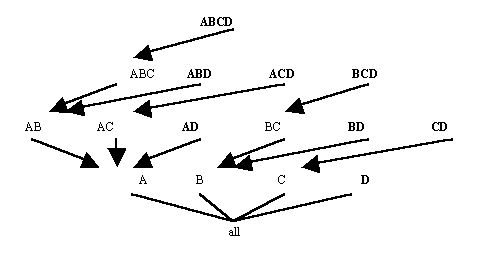
Example: Suppose the input to TDC is as shown in Table 4 and minimum support is 25% or 2 tuples. TDC first orders the database by ABCD, resulting in Table 10. After counting all combinations for ABCD, ABC, AB and A, the Iceberg-Cube is as shown in Table 11. TDC then orders the database by ABD, as shown in Table 12, and counts the combinations ABD, AB and A. The result is shown in Table 13. TDC continues with leaf nodes ACD, AD, BCD, BD, CD and D. No pruning occurs for this input table. The final result is shown in Table 14.
|
|
|
||||||||||||||||||||||||||||||||||||||||||||||||||||||||||||||||||||||||||||
|
||||||||||||||||||||||||||||||||||||||||||||||||||||||||||||||||||||||||||||||
|
|
The cardinality of an
attribute is the number of distinct values that attribute has. The TDC
algorithm prunes most efficiently when the input attributes are ordered from
highest to lowest cardinality because it is more likely to prune the first
attribute in that case.
3. Bottom-Up Computation
The bottom-up computation algorithm (BUC) repeatedly sorts the database as necessary to allow convenient partitioning and counting of the combinations without large main memory requirements. BUC begins by counting the frequency of the first attribute in the input table. The algorithm then partitions the database based on the frequent values of the first attribute, so that only those tuples that contain a frequent value for the first attribute are further examined. BUC then counts combinations of values for the first two attributes and again partitions the databse so only those tuples that contain frequent combinations of the first two attributes are further examined, and so on.
For a database with four attributes, A, B, C and D, the processing tree of the BUC algorithm is shown in Figure 12. As with the TDC processing tree, this is based on the 4-dimensional lattice from Figure 10. The algorithm examines attribute A, then partitions the database by the frequent values of A, sorting each partition by the next attribute, B, for ease of counting AB combinations. Within each partition, BUC counts combinations of attributes A and B. Again, once the frequent combinations are found, the database is partitioned, this time on frequent combinations of AB, and is sorted by attribute C. When no frequent combinations are found, the algorithm traverses back down the tree and ascends to the next node. For example, if there are no frequent combinations of AC, then BUC will examine combinations of AD next. In this way, BUC prunes passes over the data. As with the TDC algorithm, BUC prunes most efficiently when the attributes are ordered from highest to lowest cardinality.
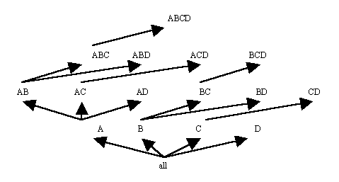
Example: Suppose the input table is as shown in Table 4 and minimum support is 25% or 2 tuples. BUC first counts A, finding the values a1 and a2 to be frequent. The ordered sets {a1, ANY, ANY, ANY} and {a2, ANY, ANY, ANY}, implicitly represented as simply {a1} and {a2}, and their frequencies are inserted into the Iceberg-Cube. BUC then partitions the database on the values a1 and a2 and sorts those partitions by attribute B. At AB, no value of B is frequent with a1. Then the a1 partition is sorted by C, but no value of C is frequent with a1. Only the combination {a1,d2} is inserted into the Iceberg-Cube after fully examining the a1 partition. BUC then examines the a2 partition, which is shown in Table 15. The combination {a2,b2} is found to be frequent and is inserted into the Iceberg- Cube. BUC then further partitions the frequent combination {a2,b2}. The new partition, as shown in Table 16, is sorted by attribute C. After counting all combinations of a2, b2 and any value for C, BUC inserts {a2,b2,c2} into the Iceberg-Cube, then creates partitions based on that combination of values. The new partitions, shown in Table 17, are sorted by attribute D. No combinations that include D are found to be frequent, so the algorithm descends the processing tree back to AB and then continues looking for combinations of ABD that include {a2,b2}. After sorting by attribute D, the partition shown in Table 18 results. Since the combination {a2,b2,d2} is frequent, it is inserted in the Iceberg-cube. No other values of D are frequent with {a2,b2}. The algorithm descends the processing tree to AB again. It continues looking for other frequent combinations of AB after {a2,b2}, but there are none, so eventually it returns to A. From A, processing continues at AC, looking for values of C that occur frequently with {a2}. The combination {a2,c2} occurs frequently, so processing ascends the tree to ACD, to look for values of D that occur frequently with {a2,c2}, but none are found. The algorithm returns to AC and then to A. From A processing continues at AD, where {a2,d2} is found to be frequent. Next the data is resorted based on the single attribute B, then combinations of attribute B and C, and so on. The final Iceberg-Cube is the same as for TDC, shown in Table 14.
Table 15: Partition of {a2} on B |
Table 16: Partition of {a2,b2} on C |
Table 17: Partition of {a2,b2,c2} on D |
Table 18: Partition of {a2,b2} on D |
4. Other Methods
For some databases the number of candidate combinations required to fit in main memory by the APRIORI algorithm becomes too large. Apart from TDC and BUC, other new methods have attempted to solve this problem. Three of these are FP-Growth, Top-k BUC and H-Mine.
FP-growth attempts to avoid candidate generation and minimize main memory use by compressing the database into a specialized data structure called an FP-tree. Unfortunately, the recursively generated conditional databases created by FP-growth may still exceed main memory size for large databases.
Top-k BUC is a specialized form of BUC, used for finding combinations with average values exceeding a specified minimum average. The average is calculated based on the sum of the values for a related measure attribute divided by the count of values. Top-k BUC also uses an H-tree (hyper-tree) for this problem.
Another recent algorithm is the H-Mine algorithm, based on partitioning
the database. This algorithm requires less main memory than APRIORI and
FP-Growth but more than BUC.
Generalization Space
Given a relation and a set of concept hierarchies, one for each attribute of the relation, the set
of possible ways of viewing the relation during summarization (rolling-up) is called the generalization space.
Assume that summarization is always done one level at a time.
The Province attribute has 4 levels in its concept hierarchy, numbered P3
(for the most specific data - the original relation) to P0 (for the single value ANY). The Amount attribute
also has 4 levels numbered A3 to A0. The resulting generalization space is shown in Figure 13. In Figure 13,
the node labelled Figure 14 shows a sample 3-dimensional generalization space.
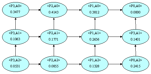
Figure 13: 2-Dimensional Generalization Space
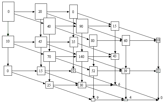
Figure 14: 3-Dimensional Generalization Space


