Notes 03-2: Distance-Based Classification

Each item that is mapped to a class may be thought of as being more similar to the other items in that class than it is to the items in other classes. Distance measures can be used to quantify the similarity of different items.

Distance Measures

A distance measure is

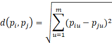
The best known distance measures are Euclidean distance and Manhattan distance. According to the Euclidean distance (or straight line distance), for some arbitrary m-dimensional instance p_i described by (p_i1, p_i2, …, p_im), where p_iu denotes the value of the u-th attribute of p_i, then the difference between two instances p_i and p_j is defined as

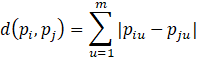
An alternative distance measure is the Manhattan distance.

k-Nearest Neighbour Technique

The k-nearest neighbour technique assumes instances can be represented by points in a Euclidean space.

The nearest neighbours of an instance are defined in terms of the standard Euclidean distance.

Example – General idea behind k-nearest neighbour classification

EXAMPLE = Classification.D.1.a

A k-nearest neighbour classifier

Algorithm: KNN

Input: D = a set of points (i.e., instances) in Euclidean space

       of the form

       k = the number of neighbours to consider

p' = an unlabeled instance

Output: C_KNN = the class label

Method:

1. j = 0

2. for each p Î D

3.     j ++

4.     if k == 1

5.         if d (p, p') <= NN [1].distance

6.             NN [1].distance = d (p, p')

7.             NN [1].class = class (p)

8.     else if j <= k

9.         i = j

10.         while i > 1 and d (p, p') <= NN [i – 1].distance

11.             NN [i].distance = NN [i – 1].distance

12.             NN [i].class = NN [i – 1].class

13.             i –-

14.         NN [i].distance = d (p, p')

15.         NN [i].class = class (p)

16.     else

17.         i = k + 1

18.         while i > 1 and d (p, p') <= NN [i – 1].distance

19.             NN [i].distance = NN [i – 1].distance

20.             NN [i].class = NN [i – 1].class

21.             i –-

22.         NN [i].distance = d (p, p')

23.         NN [i].class = class (p)

24. c = 1

25. class [c].class = NN [1].class

26. class [c].count = 1

27. for j = 2 to k

28.     newClass = true

29.     for i = 1 to c

30.         if class [i].class == NN [j].class

31.             class [i].count ++

32.             newClass = false

33.             break

34.     if newClass

35.         c ++

36.         class [c].class = NN [j].class

37.         class [c].count = 1

38. C_KNN = class [1].class

39. count = class [1].count

40. for i = 2 to c

41.     if class [c].count >= count

42. C_KNN = class [i].class

43.         count = class [i].count

Example – Predicting a class label using KNN

Tuple	Gender	Height	Class
t1	f	1.6	short
t2	m	2.0	tall
t3	f	1.9	medium
t4	f	1.8	medium
t5	f	1.7	short
t6	m	1.85	medium
t7	f	1.6	short
t8	m	1.7	short
t9	m	2.2	tall
t10	m	2.1	tall
t11	f	1.8	medium
t12	m	1.95	medium
t13	f	1.9	medium
t14	f	1.8	medium
t15	f	1.75	medium

The class label attribute is Class and has three unique values: short, medium, and tall.

The unlabeled instance to be classified is .

Assume k = 5. The five nearest neighbors to  are , , , , and . Since four out of five of the nearest neighbors are short, C_KNN = short, so we have .

Normalizing Values

Since different attributes can be measured on different scales, the Euclidean distance formula may exaggerate the effect of some attributes having larger scales. Normalization can be used to force all values to lie between 0 and 1.

where v_i is the actual value of attribute i and min(v_i) and max(v_i) are the minimum and maximum values, respectively, taken over all instances.

Example – Normalizing attribute values

Given the values 5, 3, 8, 12, 9, 15, 11, 6, and 1, the normalized values are (5–1)/(15–1) = 4/14, 2/14, 7/14, 11/14, 8/14, 14/14, 10/14, 5/14, and 0/14.