Notes 03-6: Regression
Linear regression techniques attempt to model data using a straight line.
Given a set of data points (x1, y1), (x2, y2), …, (xn, yn), where yi is some response corresponding to xi, linear regression is a method for determining the function that best fits the observed data points.
The first step in fitting a straight line to the data points is to construct a scatter plot.
If the points appear to approximate a straight line, linear regression may be an appropriate analysis technique.
DIAGRAM = Classification.C.1.b1
If they don’t, some other technique is required.
DIAGRAM = Classification.C.1.b2
The method of least squares assumes the best-fit curve is one that has the minimal sum of the deviations squared from a given set of data points.
The general regression equation can be written as
![]()
where α and β are called the regression coefficients.
The regression coefficients can be estimated from the following two equations:
![]()
![]()
Where x̅ is the mean of the x values in the sample, y̅ is the mean of the y values, β represents the slope of the line through the points, and α represents the y-intercept.
Example – Linear regression
Consider the table shown below, where Salary is shown for various values of Years of Service. The objective is to use the data in this table to predict Salary based upon Years of Service. Salary is called the explanatory variable and Years of Service is called the response variable.
|
Salary |
Years of Service |
|
30 |
3 |
|
57 |
8 |
|
64 |
9 |
|
72 |
13 |
|
36 |
3 |
|
43 |
6 |
|
59 |
11 |
|
90 |
21 |
|
20 |
1 |
|
83 |
16 |
A scatter plot corresponding to the values in the table is shown below.
DIAGRAM = Classification.C.1.d
Based upon the values in the table, x̅ = 9.1, y̅ = 55.4, β = 3.54, and α = 23.19. Therefore ŷ = 23.19 + 3.54x.
Salary can now predicted for any value of Years of Service. However, keep in mind that it is just a prediction. For example, the actual versus predicted Salary for Years of Service from the original table is shown below.
|
Salary |
Years of Service |
|
|
30 |
3 |
33.81 |
|
57 |
8 |
51.51 |
|
64 |
9 |
55.05 |
|
72 |
13 |
69.21 |
|
36 |
3 |
33.81 |
|
43 |
6 |
44.43 |
|
59 |
11 |
62.13 |
|
90 |
21 |
97.53 |
|
20 |
1 |
26.73 |
|
83 |
16 |
79.83 |
When interpreting the regression coefficients:
The estimated slope β = 3.54 implies that each additional year of service results in an increase in salary of $3,450.
The regression line should not be used to predict the response ŷ when x lies outside the range of the initial values.
Example
DIAGRAM = Classification.C.1.e
Coefficient of Determination
The coefficient of determination represents the proportion of the total variability that is explained by the model.
The coefficient of determination is represented by
![]()
where the numerator is the measure of the total variability of the fitted values and the denominator is the measure of the total variability of the original values.
A value close to 1 implies that most of the variability is explained by the model.
A value close to 0 implies that the model is not appropriate.
Naïve Bayes
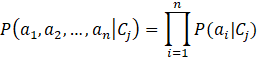
The Naïve Bayes classifier is a well-known and highly effective classifier based upon Bayes’ Rule, a technique used to estimate the likelihood of class membership of an unseen instance given the set of labeled instances.
The prior (or unconditional) probability, P(a), associated with a proposition a (i.e., an assertion that a is true) is the degree of belief accorded to it in the absence of any other information.
Example – Prior probability
P(rain = true) = 0.25 or P(rain) = 0.25
The posterior (or conditional) probability, P(a | b), associated with a proposition a is the degree of belief accorded to it given that all we know is b.
Example – Posterior probability
P(rain | thunder) = 0.8
A prior probability, such as P(rain), can be thought of as a special case of the posterior probability P(rain | ), where the probability is conditioned on no evidence.
Posterior probabilities can be defined in terms of prior probabilities. Specifically,
![]()
for P(b) > 0, which can also be written as
![]()
In a nutshell: For a and b to be true, we need b to be true, and we need a to be true given b.
Since conjunction is commutative ![]() , so
, so
![]()
can be written equivalently as
![]()
Then, since ![]() , we have Bayes’ Rule
, we have Bayes’ Rule
![]()
which can be written as
![]()
A Naïve Bayes classifier applies to
classification tasks where each instance x is described by a conjunction
of attribute values (i.e., a tuple ![]() ) and where the target class can take on any value from some finite
set C (i.e., the set of possible class values).
) and where the target class can take on any value from some finite
set C (i.e., the set of possible class values).
A set of labeled instances is provided from which the prior and posterior probabilities can be derived.
Predicting with Naïve Bayes
When a new instance is presented, the classifier is asked to predict the class label.
The Bayesian approach considers a set of candidate hypotheses (i.e., the various possible class labels) and determines the hypothesis (i.e., the class label) that is most probable given the labeled instances (known as the maximum posteriori hypothesis (MAP)).
Given a new instance with attribute values ![]() , the most probable class label is given by
, the most probable class label is given by
![]()
Using Bayes’ Rule, the above expression can be written as
![]()
or
![]()
That is, the denominator ![]() can be dropped because it is a constant
term independent of Cj.
can be dropped because it is a constant
term independent of Cj.
Since a Naïve Bayes classifier assumes the
effect of an attribute value on a given class is independent of the values of
the other attributes (called the class conditional independence assumption),
given CMAP, the probability of observing the conjunction ![]() is just the product of the probabilities of the individual
attributes. That is,
is just the product of the probabilities of the individual
attributes. That is,
Substituting ![]() for
for ![]() in the equation for CMAP yields
in the equation for CMAP yields
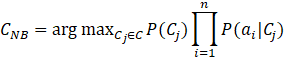
where CNB denotes the assigned class label output by the Naïve Bayes classifier.
Naïve Bayes Classifier for Categorical Attributes
Algorithm: Naïve Bayes Learner
Input:
D = a set of
labeled instances of the form ![]() ,
,
where each ai corresponds to a value from the domain of
attributes A1, A2, ..., An, respectively, and an is the
assigned class label
Output: classProbability = an array of prior probabilities
attributeProbability = an array of posterior probabilities
v = an array of the number of unique values in the domain of each attribute
Method:
1. totalCount = 0
2. m = the number of unique classes in the domain of An
3. n = the number of attributes in the instances of D
4. for j = 1 to m
5. classCount [j] = 0
6. for i = 1 to n - 1
7. v [i] = the number of unique values in the domain of Ai
8. for k = 1 to v [i]
9. attributeCount [j, i, k] = 0
10. for each instance of D
11. totalCount ++
12. j = an integer corresponding to the class of the current instance
13. classCount [j] ++
14. for i = 1 to n - 1
15. k = an integer corresponding to the value of the current attribute
16. attributeCount [j, i, k] ++
17. for j = 1 to m
18. classProbability [j] = classCount [j] / totalCount
19. for i = 1 to n
20. for k = 1 to v [i]
21. attributeProbability [j, i, k] = attributeCount [j, i, k] / classCount [j]
Algorithm: NaiveBayesClassifier
Input: classProbability = an array of prior probabilities
attributeProbability = an array of posterior probabilities
m = the number of unique classes in the domain of An
n = the number of attributes in the instances of D
v = an array of the number of unique values in the domain of each attribute
![]() = an unlabeled
instance
= an unlabeled
instance
Output: CNB = the class label
Method:
1. CNB = 0
2. for j = 1 to m
3. CTemp = classProbability [j]
4. for i = 1 to n - 1
5. for k = 1 to v [i]
6. if ai == the attribute value corresponding to v [i]
7. CTemp = CTemp * attributeProbability [j, i, k]
8. break
9. if CTemp > CNB
10. CNB = CTemp
Example – Predicting a class label using a Naïve Bayes classifier
|
Tuple |
Age |
Income |
Student |
Credit Rating |
Buys Computer |
|
t1 |
<=30 |
high |
no |
fair |
no |
|
t2 |
<=30 |
high |
no |
excellent |
no |
|
t3 |
31..40 |
high |
no |
fair |
yes |
|
t4 |
>40 |
medium |
no |
fair |
yes |
|
t5 |
>40 |
low |
yes |
fair |
yes |
|
t6 |
>40 |
low |
yes |
excellent |
no |
|
t7 |
31..40 |
low |
yes |
excellent |
yes |
|
t8 |
<=30 |
m |
no |
fair |
no |
|
t9 |
<=30 |
low |
yes |
fair |
yes |
|
t10 |
>40 |
medium |
yes |
fair |
yes |
|
t11 |
<=30 |
medium |
yes |
excellent |
yes |
|
t12 |
31..40 |
medium |
no |
excellent |
yes |
|
t13 |
31..40 |
high |
yes |
fair |
yes |
|
t14 |
>40 |
medium |
no |
excellent |
no |
The class label attribute is Buys Computer and it has two unique values: yes and no. The unlabeled instance to be classified is
áAge = “<=30”, Income = medium, Student = yes, Credit Rating = fairñ.
Let a1
= “<=30”, a2 = medium, a3 = yes,
and a4 = fair. So, the problem is to determine ![]() for all j. Now,
for all j. Now,
P(C1) = P(Buys Computer = yes) = 9/14
and
P(C2) = P(Buys Computer = no) = 5/14.
To determine CNB, we only need to concern ourselves with the conditional probabilities associated with the attribute values on the unlabeled instance. So,
![]() = P(C1) P(a1|C1)
P(a2|C1) P(a3|C1)
P(a4|C1)
= P(C1) P(a1|C1)
P(a2|C1) P(a3|C1)
P(a4|C1)
= (9/14)(2/9)(4/9)(6/9)(6/9)
= (0.643)(0.222)(0.444)(0.667)(0.667)
= 0.028
and
![]() = P(C2)
P(a1|C2) P(a2|C2)
P(a3|C2) P(a4|C2)
= P(C2)
P(a1|C2) P(a2|C2)
P(a3|C2) P(a4|C2)
= (5/14)(3/5)(2/5)(1/5)(2/5)
= (0.357)(0.6)(0.4)(0.2)(0.4)
= 0.007
We need to
maximize ![]() . Therefore, CNB = C1 = (Buys
Computer = yes).
. Therefore, CNB = C1 = (Buys
Computer = yes).