Notes 04-2: Decision Tree Construction
A decision tree is constructed by looking for regularities in data.
From Data to Trees: Quinlan's ID3 Algorithm for Constructing a Decision Tree
General Form:
Until each leaf node is populated by as homogeneous a sample set as possible:
· Select a leaf node with an inhomogeneous sample set.
· Replace that leaf node by a test node that divides the inhomogeneous sample set into minimally inhomogeneous subsets, according to an entropy calculation.
Specific Form:
1. Examine the attributes to add at the next level of the tree using an entropy calculation.
2. Choose the attribute that minimizes the entropy.
Tests Should Minimize Entropy
It is computationally impractical to find the smallest possible decision tree, so we use a procedure that tends to build small trees.
Choosing an Attribute using the Entropy Formula
The central focus of the ID3 algorithm is selecting which attribute to test at each node in the tree.
Procedure:
1. See how the attribute distributes the instances.
2. Minimize the average entropy.
· Calculate the average entropy of each test attribute and choose the one with the lowest degree of entropy.
Review of Log2
On a calculator:
![]()
eg) (0)log2(0) = -∞ (the formula is no good for a probability of 0)
eg) (1)log2(1) = 0
eg) log2(2) = 1
eg) log2(4) = 2
eg) log2(1/2) = -1
eg) log2(1/4) = -2
eg) (1/2)log2(1/2) = (1/2)(-1) = -1/2
Entropy
Given D, a collection of instances, entropy is defined as
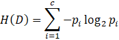
where c is the number of possible class labels contained in D and pi is the proportion of instances of D belonging to class i.
Example – Calculating entropy for data containing three classes
Suppose D is a collection of 18 examples, where the number of instances in C1 is 9, in C2 is 5, and in C3 is 4. Then the entropy of D is
![]()
Entropy has the properties that H(D) = 0 if all instances of D belong to the same class, and H(D) = log2 c if there is an equal number of instances of D in each class.
Entropy, a measure from information theory, characterizes the (im)purity, or homogeneity, of an arbitrary collection of examples.
Given:
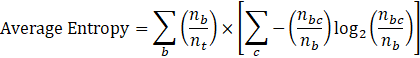
· nb, the number of instances in branch b.
· nbc, the number of instances in branch b of class c. Of course, nbc is less than or equal to nb
· nt, the total number of instances in all branches.
Probability:
![]()
![]()
· If all the instances on the branch are positive, then Pb = 1 (homogeneous positive)
· If all the instances on the branch are negative, then Pb = 0 (homogeneous negative)
Entropy:
![]()
· As you move from perfect balance and perfect homogeneity, entropy varies smoothly between zero and one.
o The entropy is zero when the set is perfectly homogeneous.
o The entropy is one when the set is perfectly inhomogeneous.
The disorder in a set containing members of two classes A and B, as a function of the fraction of the set beloning to class A.
In the diagram above, the total number of instances in both classes combined is two.
In the diagram below, the total number of instances in both classes is eight.
Average Entropy:
Information Gain
Information gain is a common method used to determine the attribute that will best classify the instances.
Information gain is defined in terms of entropy, a measure used in information theory that characterizes the “impurity” of an arbitrary collection of instances.
Information gain is the expected reduction in entropy caused by partitioning the instances according to some attribute Ai and is defined as
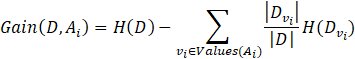
where Values(Ai)
is the set of all possible values for attribute Ai, and ![]() is the set of instances in D for
which vi is the value of Ai. The first
term, H(D), is just the entropy of the original collection of
instances in D. The second term is just the sum of the entropies of each
subset
is the set of instances in D for
which vi is the value of Ai. The first
term, H(D), is just the entropy of the original collection of
instances in D. The second term is just the sum of the entropies of each
subset ![]() , weighted by the fraction of examples in D that belong to
, weighted by the fraction of examples in D that belong to ![]() .
.
ID3 Algorithm
The ID3 tree induction algorithm (a basic form of the algorithm used in C4.5/5.0).
Algorithm: ID3
Input: D = the training data
A = the set of attributes to be tested
Ap = the attribute whose value is to be predicted
Output: CID3 = the root of the decision tree
1. create a node L
2. if all instances of D are of the same class
3. return L as a leaf node labeled with this class
4. if |A| == 0
5. return L as a leaf node labeled with the most common class in D
6. Ai = the attribute in A that best classifies the instances
7. label L with Ai
8. for each unique ai of Ai
9. add a branch below L corresponding to the case where ai is the value of Ai
10. let ![]() be the set of
instances in D where ai is the value of Ai
be the set of
instances in D where ai is the value of Ai
11. if |![]() | == 0
| == 0
12. add a leaf node labeled with the most common class in D
13. else
14. add the
node returned by ID3 (![]() , A – {Ai}, Ap)
, A – {Ai}, Ap)
15. CID3 = L
Comments on the ID3 Algorithm
Unlike the version space candidate-elimination algorithm,
· ID3 searches a completely expressive hypothesis space (ie. one capable of expressing any finite discrete-valued function), and thus avoids the difficulties associated with restricted hypothesis spaces.
· ID3 searches incompletely through this space, from simple to complex hypotheses, until its termination condition is met (eg. until it finds a hypothesis consistent with the data).
· ID3's inductive bias is based on the ordering of hypotheses by its search strategy (ie. follows from its search strategy).
· ID3's hypothesis space introduces no additional bias.
Inductive bias of ID3: shorter trees are preferred over larger trees. Also, trees that place attributes which lead to more information gain (attributes that sort instances to most decrease entropy) are placed closer to the root of the tree.
ID3's capabilities and limitations stem from its search space and search strategy:
· ID3 searches a complete hypothesis space, meaning that every finite discrete-valued function can be represented by some decision tree.
o Therefore, ID3 avoids the possibility that the target function might not be contained within the hypothesis space (a risk associated with restriction bias algorithms).
· As ID3 searches through the space of decision trees, it maintains only a single current hypothesis.
o This contrasts with the candidate-elimination algorithm, which finds all hypotheses consistent with the training data.
o By learning only a single hypothesis, ID3 loses benefits associated with explicitly representing all consistent hypotheses.
§ For instance, it does not have the ability to determine how many decision trees that are consistent with the data could exist, or select the best hypothesis among these.
· In its pure form, ID3 performs no backtracking in its search (greedy algorithm).
o Once an attribute has been chosen as the node for a particular level of the tree, ID3 does not reconsider this choice.
o It is subject to risks associated with hill-climbing searches that do not backtrack. It may converge to a locally optimal solution that is not globally optimal.
o (Although the pure ID3 algorithm does not backtrack, we discuss an extension that adds a form of backtracking: post-pruning the decision tree.)
· At every step, ID3 refines its current hypothesis based on statistical analysis of all training examples.
o This differs from methods (such as candidate-elimination) that consider each training example individually, thus making decisions incrementally.
o Using statistical properties of all the examples is what helps to make ID3 a robust algorithm. It can be made insensitive to errors in training examples and handle noisy data by modifying its termination criteria to accept hypotheses that imperfectly fit the training data.