Notes 06-2: Similarity and Distance Measures

Distance Formulae

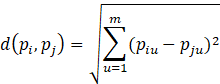
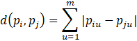
Recall that the distance or dissimilarity between two m-dimensional objects p_i = (p_i1, p_i2, …, p_im) and p_j = (p_j1, p_j2, …, p_jm) can be determined using the Euclidean Distance Function and the Manhattan Distance Function.

Euclidean Distance Formula:

Manhattan Distance Formula:

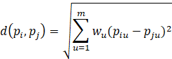
Two other distance functions are the Minkowski (a generalization of Euclidean and Manhattan distance) and Weighted Euclidean.

Minkowski Distance Formula:

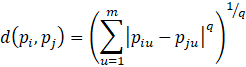
where q is a positive integer.

Note: When q = 1, Minkowski = Manhattan and when q = 2, Minkowski = Euclidean.

Weighted Euclidean Distance Formula:

Interval Scale Attributes

Interval scale attributes contain continuous measurements from a (roughly) linear scale (e.g., weight, height, temperature, latitude/longitude).

The measurement unit used can affect cluster quality (e.g., expressing an attribute in smaller units can lead to a wider range).

To minimize dependence on units, data can be standardized to give all attributes equal weight, where one approach is to convert the original measurements to a unitless attribute as follows:

First calculate the mean absolute deviation

where x₁, x₂, …, x_n are the n original measurements and x̄ is the mean value of x₁, x₂, …, x_n.

Then calculate the z-score (i.e., the standardized measurement), where each

Binary Attributes

Binary attributes have only two states: 0 meaning some condition is absent and 1 meaning it is present.

The dissimilarity between two binary attributes can be represented using a 2 by 2 contingency table (i.e., a 2 by 2 data matrix).

	Object pj
Object pi		1	0	Σ
	1	q	r	q + r
	0	s	t	s + t
	Σ	q + s	r + t	q + r + s + t

Binary attributes can be either symmetric or asymmetric.

A symmetric binary attribute assigns the same weight to both of its states (e.g., a Gender attribute having values male and female).

Similarity based on a symmetric binary attribute is called invariant similarity.

For invariant similarity, the simple matching coefficient is a well-known measure for assessing the dissimilarity between objects, and is defined as

An asymmetric binary attribute assigns different weights to its states, and by convention assigns 1 to the most important outcome (e.g., HIV positive = 1 versus HIV negative = 0 for a disease attribute).

Similarity based on an asymmetric attribute is called noninvariant similarity.

For noninvariant similarity, the Jaccard coefficient is used because it ignores t, the number of negative matches, and is defined as

Example – Dissimilarity between binary attributes

Name	Gender	Fever	Cough	Test 1	Test 2	Test 3	Test 4
Jack	m	y	n	y	n	n	n
Mary	f	y	n	y	n	y	n
Jim	m	y	y	n	n	n	n

Assume the Gender attribute is symmetric and the remaining attributes are asymmetric. The task is to calculate the dissimilarity between each pair of patients (i.e., the Jaccard coefficient will be used).

	Mary
Jack		1	0	Σ
	1	2	0	2
	0	1	3	4
	Σ	3	3	6

	Jim
Jack		1	0	Σ
	1	1	1	2
	0	1	3	4
	Σ	2	4	6

	Jim
Mary		1	0	Σ
	1	1	2	3
	0	1	2	3
	Σ	2	4	6

Using the Jaccard coefficient, the distance between each pair of patients is

d(Jack, Mary) = (0 + 1) / (2 + 0 + 1) = 0.33,

d(Jack, Jim) = (1 + 1) / (1 + 1 + 1) = 0.67, and

d(Mary, Jim) = (2 + 1) / (1 + 2 + 1) = 0.75.

Nominal Scale Attributes

Nominal scale attributes are a generalization of binary attributes where the attribute can take on more than two states (e.g., the domain values for the state of a traffic light are {green, amber, red}).

States and state labels do not imply or represent any specific ordering of the domain values.

The simple matching measure quantifies the dissimilarity between objects p_i and p_j, and is defined as

where m is the total number of attributes and q is the number of matches (i.e., the number of attributes for which p_i and p_j are in the same state).

Example – The simple matching measure

	Mary
Jack		1	0	Σ
	1	2	0	2
	0	1	3	4
	Σ	3	3	6

d(Jack, Mary) = (6 – 5) / 6 = 0.17.

Nominal scale attributes can be encoded as asymmetric binary attributes, where a new binary attribute is created for each of the nominal states.

Light	→	redLight	yellowLight	greenLight
red		1	0	0
green		0	0	1
yellow		0	1	0
green		0	0	1
red		1	0	0

Ordinal Scale Attributes

Ordinal scale attributes resemble nominal scale attributes except that the state values represent some meaningful order.

Discrete ordinal attributes describe subjective assessment of qualities that cannot be measured objectively.

domain (Professor) = {assistant, associate, full}

Continuous ordinal attributes describe a set of continuous data where the ordering of values is essential but the actual magnitude is not.

domain (Medal) = {bronze, silver, gold}

Ordinal attributes can also be obtained from interval scale attributes by splitting the range of values into a finite number of classes.

The values of ordinal attributes can be mapped to ranks.

rank (bronze) = 3

rank (silver) = 2

rank (gold) = 1

Distance measures for interval scale attributes can be used to determine the distance between ordinal attributes if the ordinal attributes are first converted to ranks.

Assume attribute u has h ordered states representing the ranks 1, …, h.

First, replace each p_iu (i.e., the value of u for the i-th object) by its corresponding rank r_iu.

Then, if it is important for each attribute to have equal weight, replace the rank r_iu with a normalized rank z_iu (i.e., it will fall in the interval [0, 1]), where

Ratio Scale Attributes

Ratio scale attributes contain measurements from a nonlinear scale (e.g., bacterial growth, radioactive decay) and may have to be converted to interval scale attributes before determining the dissimilarity between objects.

A logarithmic transformation can be used to convert a ratio scale attribute to an interval scale attribute according to the formula

y_iu = log (x_iu),

where x_iu is the ratio scale value of the i-th object for attribute u, and y_iu is the interval scale value.

A transformation from a ratio scale attribute to an interval scale attribute can be done by treating the ratio scale values as ordinal scale values and their ranks as interval scale values.

Mixed Attribute Types

In real databases, objects are described by a mixture of attribute types and dissimilarity can be assessed by normalizing the meaningful attributes onto the interval [0, 1] and combining the different attributes into a single dissimilarity matrix.

Assume a database of m attributes of mixed types.

The dissimilarity of objects p_i and p_j in dataset D is defined as

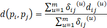
where δ_ij^(u) = 0 if either p_iu or p_ju is missing (i.e., there is no value recorded for attribute u for object p_i or p_j), or p_iu = p_ju = 0 and attribute u is asymmetric binary; otherwise δ_ij^(u) = 1. The contribution of attribute u to the dissimilarity between p_i and p_j is d_ij^(u) and is dependent on its type. That is,

If u is binary or nominal:

d_ij^(u) = 0 if p_iu = p_ju;

Otherwise d_ij^(u) = 1.

If u is interval-scaled:

where max and min consider all objects that have a value for attribute u.

If u is ordinal or ratio scaled: Convert each p_iu to rank r_iu, determine z_iu and treat z_iu as an interval-scaled attribute.