Reference:

• D. Schuurmans, Machine Learning course notes, University of Waterloo, 1999.
• T. Mitchell, Machine Learning, McGraw-Hill, 1997, pp. 20-50.

Machine learning is a process which causes systems to improve with experience.

Elements of a Learning Task

Representation

1. Items of Experience
   • i I
2. Space of Available Actions
   • a A
3. Evaluation
   • v (a, i)
4. Base Performance System
   • b: I A
5. Learning System
   • L: (i₁, a₁, v₁)...(i_n, a_n, v_n) b
   • Maps training experience sequence to base performance system.

Types of Learning Problems

Fundamental Distinctions

• Between problems rather than methods.
• Influences choice of method.

1. Batch versus Online Learning:
   • Batch Learning
     • Training phase (no responsibility for performance during learning), then testing.
     • Synthesizing a base performance system.
     • Pure exploration.
   • Online Learning
     • No separate phase.
     • Learning while doing.
     • Have to decide between choosing actions to perform well now versus gaining knowledge to perform well later.
2. Learning from Complete versus Partial Feedback:
   • Complete Feedback
     • Each item of experience evaluates every action (or base system).
     • Tells what best action would have been.
   • Partial Feedback
     • Each item of experience evaluates only a subset of possible actions (or base systems).
     • Only tells you how you did.
     • Creates exploration/exploitation tradeoff in online setting.
       • Should the reward be optimized with what is already known or should learning be attempted?
       • In batch learning, exploration would be chosen since there is no responsibility for performance.
   • Pointwise Feedback
     • Evaluates single action.
       • Optimization problem: (Controller, State) Action.
3. Passive versus Active Learning
   • Passive: observation.
   • Active: experimentation, exploitation.
4. Learning in Acausal versus Causal Situations
   • Acausal: actions do not affect future experience.
     • e.g., rain prediction
   • Causal: actions do effect future experience.
5. Learning in Stationary versus Nonstationary Environments
   • Stationary: evaluation doesn't change.
   • Nonstationary: evaluation changes with time.

Concept Learning

The problem of inducing general functions from specific training examples is central to learning.

Concept learning acquires the definition of a general category given a sample of positive and negative training examples of the category, the method of which is the problem of searching through a hypothesis space for a hypothesis that best fits a given set of training examples.

A hypothesis space, in turn, is a predefined space of potential hypotheses, often implicitly defined by the hypothesis representation.

Learning a Function from Examples

• An example of concept learning where the concepts are mathematical functions.

Given:

• Domain X: descriptions
• Domain Y: predictions
• H: hypothesis space; the set of all possible hypotheses
• h: target hypothesis

Idea: to extrapolate observed y's over all X.

Hope: to predict well on future y's given x's.

Require: there must be regularities to be found!

(Note type: batch, complete, passive (we are not choosing which x), acausal, stationary).

Many Research Communities

• Representation choice differs.
• Prefer maximum level of abstraction.

Traditional Statistics

• h: Rⁿ R
• Squared prediction error.
• h is a linear function.

Traditional Pattern Recognition

• h: R {0, 1}
• Right/wrong prediction error.
• h is a linear discriminant boundary.

"Symbolic" Machine Learning

• h: {attribute-value vectors} {0, 1}
• h is a simple boolean function (eg. a decision tree).

Neural Networks

• h: Rⁿ R
• h is a feedforward neural net.

Inductive Logic Programming

• h: {term structure} {0, 1}
• h is a simple logic program.

Learning Theory

• Postulate mathematical model of learning situations.
• Rigorously establish achievable levels of learning performance.
• Characterize/quantify value of prior knowledge and constraints.
• Identify limits/possibilities of learning algorithms.

Standard Learning Algorithm

Given a batch set of training data S = {(x₁, y₁)...(x_t, y_t)}, consider a fixed hypothesis class H and compute a function h H that minimizes empirical error.

Example: Least-Squares Linear Regression

Here, the standard learning algorithm corresponds to least squares linear regression.

X = Rⁿ, Y = R

H = {linear functions Rⁿ R}

Choosing a Hypothesis Space

In practice, for a given problem X Y, which hypothesis space H do we choose?

Question: since we know the true function f: X Y, should we make H as "expressive" as possible and let the training data do the rest?

• e.g., quadratic
• e.g., high degree polynomial
• e.g., complex neural network.

Answer: no!
Reason: overfitting!

• Underfit
  • Unable to express a good prediction.
• Overfit
  • Hard to identify good from bad candidates.

Basic Overfitting Phenomenon

Overfitting is bad.

Example: polynomial regression

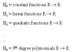
Suppose we use a hypothesis space, with many classes of functions

Given n = 10 training points (x₁, y₁)...(x₁₀, y₁₀).

Since n = 10, with 10 pieces of data, then in

there is a function that gives an exact fit.

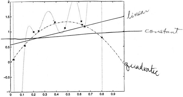
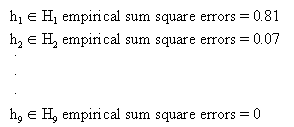
Which hypothesis would predict well on future examples?

• Although hypothesis h₉ fits these 10 data exactly, it is unlikely to fit the next piece of data well.

When does empirical error minimization overfit?

Depends on the relationship between

• hypothesis class, H
• training sample size, t
• data generating process