Least Squares Estimation of Derivatives

I have explored two least Squares methods for estimating the derivaties at a point on a functional mesh using local mesh points. The first uses only regular or equally weighted Least Squares fitting. The second uses Weighted Least Squares where the weight assigned to a mesh point is given by a tight gaussian function centered around the point for which the estimation is being made. Early work demonstrated that the matrices used for fitting surfaces are poorly conditioned unless they are overconstrained (M >> N). However, overconstraining means that data points which lie far from the region of interest are used resulting in a poorly fitted surface. Thinking that the poor conditioning resulted from my naive use of the power polynomial basis, I decided to try the bernstein basis in the range 0-1 which some papers indicated was generally better conditioned. The conditioning numbers I got as a result were about a constant multiple of 3 better than with the power basis in the domain (0-1,0-1) and far better outside that domain, but I still get a conditioning number of about 10^4. Randomly perturbing the mesh points seems to lead to better conditioned matrices when the conditioning number for a regular grid is critically bad (10^10 - 10^17), but the surfaces still look odd. So I tried using Weighted Least Squares, but found that my results were not a lot better unless I weighted the points immediately adjacent to the point of interest much more than the rest.The following images illustrate some of the results I am seeing.

S3d Files comparing Clough/Tocher and my efforts

1st-5th	1st-4th	1st-3rd
1st-2nd	1st	None

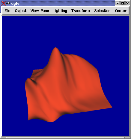
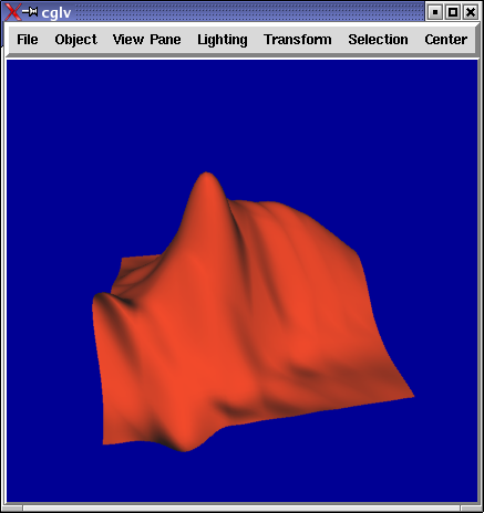
Accurate computed derivatives per vertex. My estimations seem to fit between accurate 1st and accurate 1&2nd. Some results with weighted least squares are similar in appearance to 1st&2nd&3rd. Comparison is difficult, however, because these renderings use a different sampling than my new ones.

Estimation Work

All pictures use same domain, (-1,-1) -> (1,1), and a sampling of 11x11 on the Franke function. Random images use perturbation of .1.

First Monomial fit. Uses 5th degree approximation and uses a 6x6 grid of points (36 points) where only 21 should be necessary.


Monomial fit with randomly perturbed points. Uses 5th degree approximation and uses a 5x5 grid of points (25 points) where only 21 should be necessary. Without random perturbation the surface is impossible to render. Left: unweighted Right:weighted. Images are random and difficult to compare.


First Bernstein fit. Uses 5th degree approximation and a 6x6 grid of points (36 points) where only 21 should be necessary.


Weighted fit comparison. Uses 5th degree approximation and a 6x6 grid of points (36 points) where only 21 should be necessary. From right to left the weighting function is pseudo-gaussian bell double degree, degree, half degree, and quarter degree in diameter before plateauing.


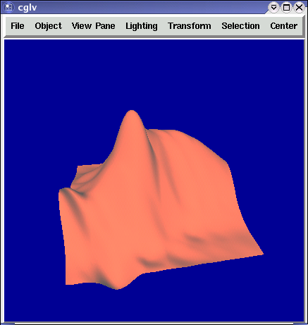
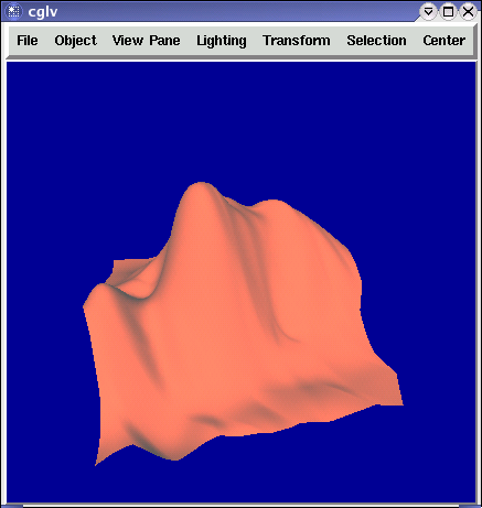
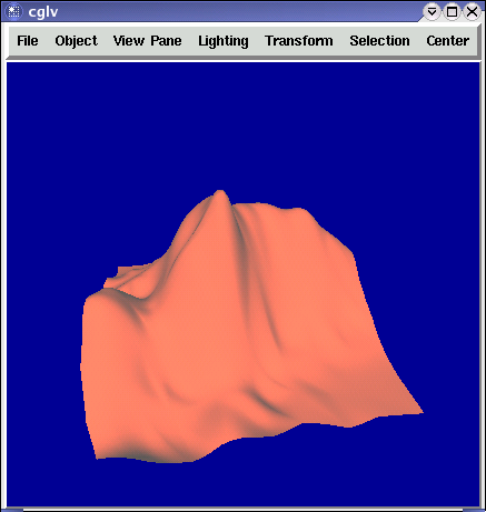
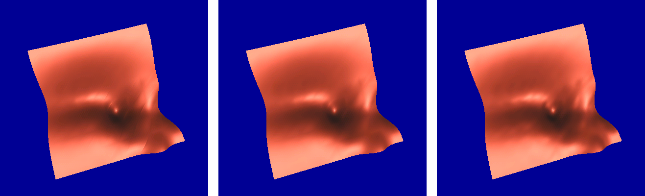
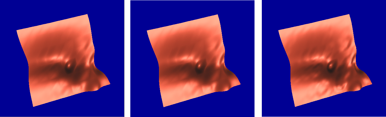
Weighted phong shaded results, all with degree 5 approximation. left: No continuity correction, degree 5 patch. center: C1 correction, degree 5 patch. right C2 correction, degree 9 patch.


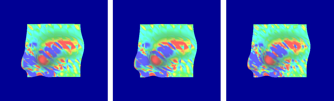
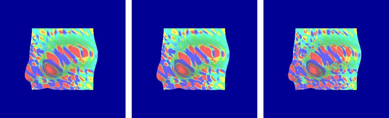
Weighted gaussian curvature shaded results, all with degree 5 approximation. left: No continuity correction, degree 5 patch. center: C1 correction, degree 5 patch. right C2 correction, degree 9 patch.


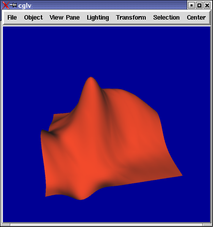
Unweighted phong shaded results, all with degree 5 approximation. left: No continuity correction, degree 5 patch. center: C1 correction, degree 5 patch. right C2 correction, degree 9 patch.


Unweighted gaussian curvature shaded results, all with degree 5 approximation. left: No continuity correction, degree 5 patch. center: C1 correction, degree 5 patch. right C2 correction, degree 9 patch.