Introduction
Users of decision support systems often see data in the form of data cubes. The cube is used to represent data along some measure of interest. Although called a "cube", it can be 2-dimensional, 3-dimensional, or higher-dimensional. Each dimension represents some attribute in the database and the cells in the data cube represent the measure of interest. For example, they could contain a count for the number of times that attribute combination occurs in the database, or the minimum, maximum, sum or average value of some attribute. Queries are performed on the cube to retrieve decision support information.
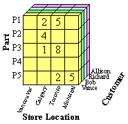 |
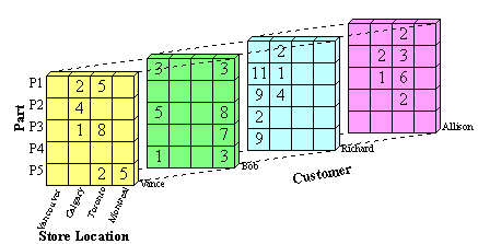 |
| Figure 1(a): Front View of Sample Data Cube |
Figure 1(b): Entire View of |
Computed versus Stored Data Cubes
The goal is to retrieve the decision support information from the data cube in the most efficient way possible. Three possible solutions are:
- Pre-compute all cells in the cube
- Pre-compute no cells
- Pre-compute some of the cells
If the whole cube is pre-computed, then queries run on the cube will be very fast. The disadvantage is that the pre-computed cube requires a lot of memory. The size of a cube for n attributes A1,...,An with cardinalities |A1|,...,|An| is π|Ai|. This size increases exponentially with the number of attributes and linearly with the cardinalities of those attributes.
To minimize memory requirements, we can pre-compute none of the cells in the cube. The disadvantage here is that queries on the cube will run more slowly because the cube will need to be rebuilt for each query.
As a compromise between these two, we can pre-compute only those cells in the cube which will most likely be used for decision support queries. The trade-off between memory space and computing time is called the space-time trade-off, and it often exists in data mining and computer science in general.
Representation
m-Dimensional Array:
A data cube built from m attributes can be stored as an m-dimensional array. Each element of the
array contains the measure value, such as count. The array itself can be
represented as a 1-dimensional array. For example, a 2-dimensional array of
size x x y can be stored as a 1-dimensional array of size x*y,
where element (i,j) in the 2-D array is stored in location (y*i+j)
in the 1-D array. The disadvantage of storing the cube directly as an array is
that most data cubes are sparse, so the array will contain many empty elements (zero values).
List of Ordered Sets:
To save storage space we can store the cube as a sparse array or a list of ordered sets. If we store all
cells in the data cube from Figure 1, then the resulting datacube will contain (cardPart
*cardStoreLocation*cardCustomer)
combinations, which is 5 * 4 * 4 = 80 combinations.
If we eliminate cells in the cube that contain zero, such as {P1, Vancouver, Allison}, only 27 combinations remain, as seen in Table 1.
Table 1 shows an ordered set representation of the data cube. Each attribute value combination is paired with its corresponding count. This representation can be easily stored in a database table to facilitate queries on the data cube.
|
|
Table 1: Ordered Set Representation of a Data Cube
Representation of TotalsAnother aspect of data cube representation which can be considered is the representation of totals. A simple data cube does not contain totals. The storage of totals increases the size of the data cube but can also decrease the time to make total-based queries. A simple way to represent totals is to add an additional layer on n sides of the n-dimensional datacube. This can be easily visualized with the 3-dimensional data cube introduced in Figure 1. Figure 2 shows the original cube with an additional layer on each of three sides to store total values. The totals represent the sum of all values in one horizontal row, vertical row (column) or depth row of the data cube.
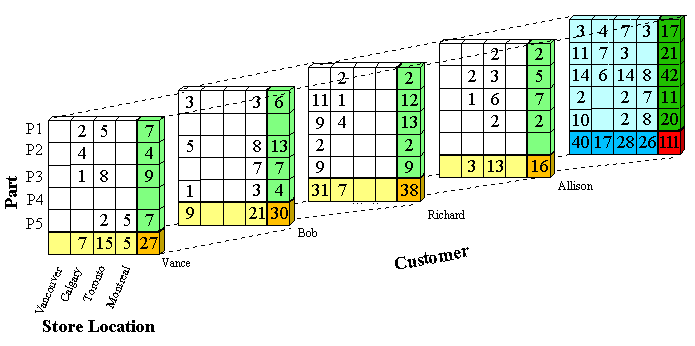
Figure 2: Cube with Totals
The color coding used in Figure 2 is as follows:
- White: Original values
- Light yellow: Total for one customer and one store location
- Light green: Total for one customer and one part
- Light blue: Total for one part and one store location
- Dark yellow: Total for one customer
- Dark green: Total for one part
- Dark blue: Total for one store location
- Red: Total number of transactions in all
To store these totals in ordered set representation the value ANY can be used. For example, there are 15 transactions where Vance buys a part in Toronto. The ordered set representation of this is ({ANY, Toronto, Vance},15), because it could be any part. The ordered set representation of all of Vance's transactions is ({ANY, ANY, Vance},27), that is all transactions at all store locations for Vance. The total number of transactions in the whole cube is found in the red cell and is 111. This is represented as ({ANY, ANY, ANY}, 111).
Operations on Data Cubes
Summarization or RollupRollup or summarization of the data cube can be done by traversing upwards through a concept hierarchy. A concept hierarchy maps a set of low level concepts to higher level, more general concepts. It can be used to summarize information in the data cube. As the values are combined, cardinalities shrink and the cube gets smaller. Generalizing can be thought of as computing some of the summary total cells that contain ANYs, and storing those in favour of the original cells.
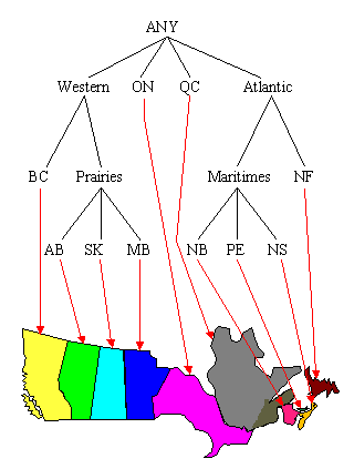
Figures 2 through 8 show an example of summarizing a data cube built from two attributes, Province and Grant_Amount. The measure of interest stored in the cube is Vote. It contains the total number of votes for each combination of Province and Grant_Amount that occurred in the input table. The concept hierarchies for the Province and Grant_Amount attributes are shown in Figure 2. In Figure 2(a), each province represents a location and some can be mapped to more general regions, such as the Prairies or the Maritimes. Those regions can be further mapped to Western Canada and Atlantic Canada. The top level of the hierarchy is "ANY", representing any location. Western and Atlantic Canada are higher level, more general concepts than, for example, Alberta and Nova Scotia. The concept hierarchy in Figure 2(b) represents the Grant_Amount dimension of the database. Grant_Amount is originally stored as specific numbers, such as $34000. The concept hierarchy generalizes the values by grouping them into categories of multiples of $10000, then $20000, and finally including all the amounts into ANY. Ordinarily, concept hierarchies are provided by a domain expert, because then the resulting general concepts will make sense to people familiar with the domain. Concept hierarchies might also be formed automatically by clustering.
 |
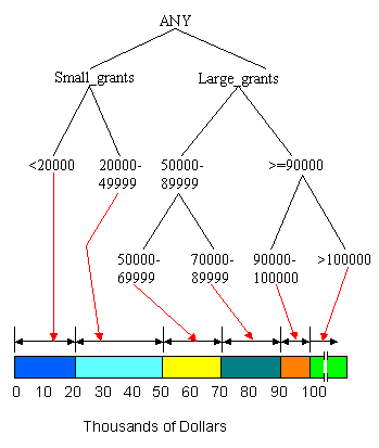 |
| Figure 2(a): Concept Hierarchy for Province | Figure 2(b): Concept Hierarchy for Grant_Amount |
To reduce the size of the data cube, we can summarize the data by computing the cube at a higher level in the concept hierarchy. A non-summarized cube would be computed at the lowest level, for example, the province level in Figure 2(a). If we compute the cube at the second level, there are only six categories, B.C., Prairies, Ont., Que., Maritimes and Nfld., and the data cube will be much smaller. Figure 3 shows a sample generalization of the Province attribute for those provinces that can be grouped under the concept Prairies and those that can be grouped under the concept Maritimes. For example, for Sask., the province, or location name, changes to Prairies, but the other attribute values remain unchanged because they are not summarized at this point. The new, summarized concept hierarchy is shown in Figure 4.
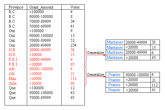
Figure 3: Generalizing the Province Attribute 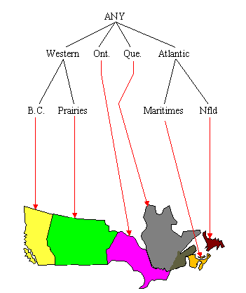
Figure 4: After Generalization of Province Attribute
The next step in the process is to remove duplicate tuples from the data. The measure of interest, Votes, is summed for tuples that have the same Province and Grant_Amount values. For example, in Figure 5, three tuples contain the combination {Prairies, <20000}. The tuples are removed, their individual Votes values are summed, and a new tuple replaces all three, with a Votes value of 231.
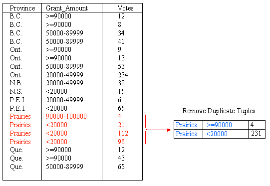
Figure 5: Remove Duplicate Tuples after Province Generalization
We can also generalize the Grant_Amount Attribute. Figure 6 shows summarization of this attribute through the addition of a new category for amounts greater than or equal to 90000. In total, the Grant_Amount value of seven tuples is changed to the new classification. After summarizing the data into groups of <20000, 20000 - 49999, 50000 -89999 and >=90000, the concept hierarchy is as shown in Figure 7. Again, we need to remove the duplicate tuples after generalizating the Grant_Amount attribute. This is shown in Figure 8.
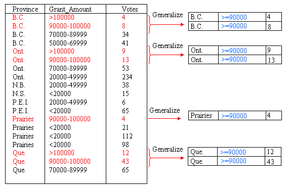
Figure 6: Generalize Grant_Amount Attribute
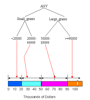
Figure 7: After Generalization of Grant_Amount Attribute
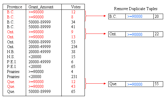
Figure 8: Removing Duplicate Tuples after Grant_Amount Generalization
The final result of summarizing the data by introducing the categories Prairies, Maritimes and >=90000 is shown in Figure 9. From here, the process could be continued to further generalize Province or Grant_Amount.
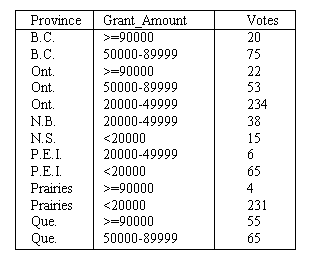
Figure 9: Final Result of Generalization
Drill-down
Drill-down is similar to Rollup, but is in reverse. A drill-down goes from less detailed data to more detailed data. To drill-down, we can either traverse down a concept hierarchy or add another dimension to the data cube. For example, given the data shown in Figure 8, a drill-down on the Province attribute would result in more detailed information about the location. The value Prairies would be replaced by the more detailed values of Alberta, Saskatchewan and Manitoba. The result is the data cube shown in Figure 7, before summarization. This is a reversal of the summarization process.


